case study on population genetics

An official website of the United States government

The .gov means it’s official. Federal government websites often end in .gov or .mil. Before sharing sensitive information, make sure you’re on a federal government site.

The site is secure. The https:// ensures that you are connecting to the official website and that any information you provide is encrypted and transmitted securely.

• Publications
• Account settings

Preview improvements coming to the PMC website in October 2024. Learn More or Try it out now .

• Advanced Search
• Journal List
• Europe PMC Author Manuscripts

Basic statistical analysis in genetic case-control studies

Geraldine m clarke.

1 Genetic and Genomic Epidemiology Unit, Wellcome Trust Centre for Human Genetics, University of Oxford, Oxford, UK.

Carl A Anderson

2 Wellcome Trust Sanger Institute, Wellcome Trust Genome Campus, Hinxton, Cambridge, UK.

Fredrik H Pettersson

Lon r cardon.

3 GlaxoSmithKline, King of Prussia, Pennsylvania, USA.

Andrew P Morris

Krina t zondervan, associated data.

This protocol describes how to perform basic statistical analysis in a population-based genetic association case-control study. The steps described involve the (i) appropriate selection of measures of association and relevance of disease models; (ii) appropriate selection of tests of association; (iii) visualization and interpretation of results; (iv) consideration of appropriate methods to control for multiple testing; and (v) replication strategies. Assuming no previous experience with software such as PLINK, R or Haploview, we describe how to use these popular tools for handling single-nucleotide polymorphism data in order to carry out tests of association and visualize and interpret results. This protocol assumes that data quality assessment and control has been performed, as described in a previous protocol, so that samples and markers deemed to have the potential to introduce bias to the study have been identified and removed. Study design, marker selection and quality control of case-control studies have also been discussed in earlier protocols. The protocol should take ~1 h to complete.

INTRODUCTION

A genetic association case-control study compares the frequency of alleles or genotypes at genetic marker loci, usually single-nucleotide polymorphisms (SNPs) (see Box 1 for a glossary of terms), in individuals from a given population—with and without a given disease trait—in order to determine whether a statistical association exists between the disease trait and the genetic marker. Although individuals can be sampled from families (‘family-based’ association study), the most common design involves the analysis of unrelated individuals sampled from a particular outbred population (‘population-based association study’). Although disease-related traits are usually the main trait of interest, the methods described here are generally applicable to any binary trait.

The result of interbreeding between individuals from different populations.

Cochran-Armitage trend test

Statistical test for analysis of categorical data when categories are ordered. It is used to test for association in a 2 × k contingency table ( k > 2). In genetic association studies, because the underlying genetic model is unknown, the additive version of this test is most commonly used.

Confounding

A type of bias in statistical analysis that occurs when a factor exists that is causally associated with the outcome under study (e.g., case-control status) independently of the exposure of primary interest (e.g., the genotype at a given locus) and is associated with the exposure variable but is not a consequence of the exposure variable.

Any variable other than the main exposure of interest that is possibly predictive of the outcome under study; covariates include confounding variables that, in addition to predicting the outcome variable, are associated with exposure.

False discovery rate

The proportion of non-causal or false positive significant SNPs in a genetic association study.

False positive

Occurs when the null hypothesis of no effect of exposure on disease is rejected for a given variant when in fact the null hypothesis is true.

Family-wise error rate

The probability of one or more false positives in a set of tests. For genetic association studies, family-wise error rates reflect false positive findings of associations between allele/genotype and disease.

Hardy-Weinberg equilibrium (HWE)

Given a minor allele frequency of p , the probabilities of the three possible unordered genotypes ( a/a , A/a , A/A ) at a biallelic locus with minor allele A and major allele a, are (1 – p ) 2 , 2 p (1 – p ), p 2 . In a large, randomly mating, homogenous population, these probabilities should be stable from generation to generation.

Linkage disequilibrium (LD)

The population correlation between two (usually nearby) allelic variants on the same chromosome; they are in LD if they are inherited together more often than expected by chance.

A measure of LD between two markers calculated according to the correlation between marker alleles.

A measure of association derived from case-control studies; it is the ratio of the odds of disease in the exposed group compared with the non-exposed.

The risk of disease in a given individual. Genotype-specific penetrances reflect the risk of disease with respect to genotype.

Population allele frequency

The frequency of a particular allelic variant in a general population of specified origin.

Population stratification

The presence of two or more groups with distinct genetic ancestry.

Relative risk

The risk of disease or of an event occurring in one group relative to another.

Single-nucleotide polymorphism (SNP)

A genetic variant that consists of a single DNA base-pair change, usually resulting in two possible allelic identities at that position.

Following previous protocols on study design, marker selection and data quality control 1 – 3 , this protocol considers basic statistical analysis methods and techniques for the analysis of genetic SNP data from population-based genome-wide and candidate-gene (CG) case-control studies. We describe disease models, measures of association and testing at genotypic (individual) versus allelic (gamete) level, single-locus versus multilocus methods of association testing, methods for controlling for multiple testing and strategies for replication. Statistical methods discussed relate to the analysis of common variants, i.e., alleles with a minor allele frequency (MAF) > 1%; different analytical techniques are required for the analysis of rare variants 4 . All methods described are proven and used routinely in our research group 5 , 6 .

Conceptual basis for statistical analysis

The success of a genetic association study depends on directly or indirectly genotyping a causal polymorphism. Direct genotyping occurs when an actual causal polymorphism is typed. Indirect genotyping occurs when nearby genetic markers that are highly correlated with the causal polymorphism are typed. Correlation, or non-random association, between alleles at two or more genetic loci is referred to as linkage disequilibrium (LD). LD is generated as a consequence of a number of factors and results in the shared ancestry of a population of chromosomes at nearby loci. The shared ancestry means that alleles at flanking loci tend to be inherited together on the same chromosome, with specific combinations of alleles known as haplotypes. In genome-wide association (GWA) studies, common SNPs are typically typed at such high density across the genome that, although any single SNP is unlikely to have direct causal relevance, some are likely to be in LD with any underlying common causative variants. Indeed, most recent GWA arrays containing up to 1 million SNPs use known patterns of genomic LD from sources such as HapMap 7 to provide the highest possible coverage of common genomic variation 8 . CG studies usually focus on genotyping a smaller but denser set of SNPs, including functional polymorphisms with a potentially higher previous probability of direct causal relevance 2 .

A fundamental assumption of the case-control study is that the individuals selected in case and control groups provide unbiased allele frequency estimates of the true underlying distribution in affected and unaffected members of the population of interest. If not, association findings will merely reflect biases resulting from the study design 1 .

Models and measures of association

Consider a genetic marker consisting of a single biallelic locus with alleles a and A (i.e., a SNP). Unordered possible genotypes are then a/a , a/A and A/A . The risk factor for case versus control status (disease outcome) is the genotype or allele at a specific marker. The disease penetrance associated with a given genotype is the risk of disease in individuals carrying that genotype. Standard models for disease penetrance that imply a specific relationship between genotype and phenotype include multiplicative, additive, common recessive and common dominant models. Assuming a genetic penetrance parameter γ (γ > 1), a multiplicative model indicates that the risk of disease is increased γ-fold with each additional A allele; an additive model indicates that risk of disease is increased γ-fold for genotype a/A and by 2γ-fold for genotype A/A ; a common recessive model indicates that two copies of allele A are required for a γ-fold increase in disease risk, and a common dominant model indicates that either one or two copies of allele A are required for a γ-fold increase in disease risk. A commonly used and intuitive measure of the strength of an association is the relative risk (RR), which compares the disease penetrances between individuals exposed to different genotypes. Special relationships exist between the RRs for these common models 9 (see Table 1 ).

Disease penetrance functions and associated relative risks.

Shown are disease penetrance functions for genotypes a/a , A/a and A/A and associated relative risks for genotypes A/a and A/a compared with baseline genotype a/a for standard disease models when baseline disease penetrance associated with genotype a/a is f 0 0 and genetic penetrance parameter is γ> 19.

RR estimates based on penetrances can only be derived directly from prospective cohort studies, in which a group of exposed and unexposed individuals from the same population are followed up to assess who develops disease. In a case-control study, in which the ratio of cases to controls is controlled by the investigator, it is not possible to make direct estimates of disease penetrance, and hence of RRs. In this type of study, the strength of an association is measured by the odds ratio (OR). In a case-control study, the OR of interest is the odds of disease (the probability that the disease is present compared with the probability that it is absent) in exposed versus non-exposed individuals. Because of selected sampling, odds of disease are not directly measurable. However, conveniently, the disease OR is mathematically equivalent to the exposure OR (the odds of exposure in cases versus controls), which we can calculate directly from exposure frequencies 10 . The allelic OR describes the association between disease and allele by comparing the odds of disease in an individual carrying allele A to the odds of disease in an individual carrying allele a . The genotypic ORs describe the association between disease and genotype by comparing the odds of disease in an individual carrying one genotype to the odds of disease in an individual carrying another genotype. Hence, there are usually two genotypic ORs, one comparing the odds of disease between individuals carrying genotype A/A and those carrying a/a and the other comparing the odds of disease between individuals carrying genotype a/A and those carrying genotype a/a. Beneficially, when disease penetrance is small, there is little difference between RRs and ORs (i.e., RR ≈ OR). Moreover, the OR is amenable to analysis by multivariate statistical techniques that allow extension to incorporate further SNPs, risk factors and clinical variables. Such techniques include logistic regression and other types of log-linear models 11 .

To work with observations made at the allelic (gamete) rather than the genotypic (individual) level, it is necessary to assume (i) that there is Hardy-Weinberg equilibrium (HWE) in the population, (ii) that the disease has a low prevalence ( < 10%) and (iii) that the disease risks are multiplicative. Under the null hypothesis of no association with disease, the first condition ensures that there is HWE in both controls and cases. Under the alternative hypothesis, the second condition further ensures that controls will be in HWE and the third condition further ensures that cases will also be in HWE. Under these assumptions, allelic frequencies in affected and unaffected individuals can be estimated from case-control studies. The OR comparing the odds of allele A between cases and controls is called the allelic RR (γ*). It can be shown that the genetic penetrance parameter in a multiplicative model of penetrance is closely approximated by the allelic RR, i.e., γ ≈ γ* ( ref. 10 ).

Tests for association

Tests of genetic association are usually performed separately for each individual SNP. The data for each SNP with minor allele a and major allele A can be represented as a contingency table of counts of disease status by either genotype count (e.g., a/a , A/a and A/A ) or allele count (e.g., a and A ) (see Box 2 ). Under the null hypothesis of no association with the disease, we expect the relative allele or genotype frequencies to be the same in case and control groups. A test of association is thus given by a simple χ 2 test for independence of the rows and columns of the contingency table.

CONTINGENCY TABLES AND ASSOCIATED TESTS

The risk factor for case versus control status (disease outcome) is the genotype or allele at a specific marker. The data for each SNP with minor allele a and major allele A in case and control groups comprising n individuals can be written as a 2 × k contingency table of disease status by either allele ( k = 2) or genotype ( k = 3) count.

Allele count

• The allelic odds ratio is estimated by OR A = m 12 m 21 m 11 m 22 .
• If the disease prevalence in a control individual carrying an a allele can be estimated and is denoted as P 0 , then the relative risk of disease in individuals with an A allele compared with an a allele is estimated by RR A = OR A 1 − P 0 + P o OR A .

An allelic association test is based on a simple χ 2 test for independence of rows and columns X 2 = ∑ i = 1 2 ∑ j = 1 2 ( m i j − E [ m i j ] ) 2 E [ m i j ] where E [ m i j ] = m i • m • j 2 n X 2 has a χ 2 distribution with 1 d.f. under the null hypothesis of no association.

Genotype count

• The genotypic odds ratio for genotype A/A relative to genotype a/a is estimated by OR A A = n 13 n 21 n 11 n 23 . The genotypic odds ratio for genotype A/a relative to genotype a/a is estimated by OR A a = n 12 n 21 n 11 n 22 .
• If the disease prevalence in a control individual carrying an a/a genotype can be estimated and is denoted as P 0 , then the relative risk of disease in individuals with an A/A [A/a] genotype compared with an a/a genotype is estimated by RR A A = OR A A 1 − P 0 + P o OR A A [ RR A a = OR A a 1 − P 0 + P o OR A a ] .
• A genotypic association test is based on a simple χ 2 test for independence of rows and columns X 2 = ∑ i = 1 2 ∑ j = 1 3 ( n i j − E [ n i j ] ) 2 E [ n i j ] where E [ n i j ] = n i • n • j n X 2 has a χ 2 distribution with 2 d.f. under the null hypothesis of no association. To test for a dominant (recessive) effect of allele A, counts for genotypes a/A and A/A ( a/a and A/a ) can be combined and the usual 1 d.f. χ 2 -test for independence of rows and columns can be applied to the summarized 2 × 2 table.
• A Cochran-Armitage trend test of association between disease and marker is given by T 2 = [ ∑ i = 1 3 w i ( n i n 2 • − n 2 n 1 • ) ] 2 n 1 • n 2 • n [ ∑ i = 1 3 w i 2 n • i ( n − n • i ) − 2 ∑ i = 1 2 ∑ j = i + 1 3 w i w j n • i n • j ] where w = ( w 1 , w 2 , w 3 ) are weights chosen to detect particular types of association. For example, to test whether allele A is dominant over allele a w = (0,1,1) is optimal; to test whether allele A is recessive to allele a , the optimal choice is w = (0,0,1). In genetic association studies, w = (0,1,2) is most often used to test for an additive effect of allele A . T 2 has a χ 2 distribut ion with 1 d.f. under the null hypothesis of no association.

In a conventional χ 2 test for association based on a 2 × 3 contingency table of case-control genotype counts, there is no sense of genotype ordering or trend: each of the genotypes is assumed to have an independent association with disease and the resulting genotypic association test has 2 degrees of freedom (d.f.). Contingency table analysis methods allow alternative models of penetrance by summarizing the counts in different ways. For example, to test for a dominant model of penetrance, in which any number of copies of allele A increase the risk of disease, the contingency table can be summarized as a 2 × 2 table of genotype counts of A/A versus both a/A and a/a combined. To test for a recessive model of penetrance, in which two copies of allele A are required for any increased risk, the contingency table is summarized into genotype counts of a/a versus a combined count of both a/A and A/A genotypes. To test for a multiplicative model of penetrance using contingency table methods, it is necessary to analyze by gamete rather than individual: a χ 2 test applied to the 2 × 2 table of case-control allele counts is the widely used allelic association test. The allelic association test with 1 d.f. will be more powerful than the genotypic test with 2 d.f., as long as the penetrance of the heterozygote genotype is between the penetrances of the two homozygote genotypes. Conversely, if there is extreme deviation from the multiplicative model, the genotypic test will be more powerful. In the absence of HWE in controls, the allelic association test is not suitable and alternative methods must be used to test for multiplicative models. See the earlier protocol on data quality assessment and control for a discussion of criteria for retaining SNPs showing deviation from HWE 3 . Alternatively, any penetrance model specifying some kind of trend in risk with increasing numbers of A alleles, of which additive, dominant and recessive models are all examples, can be examined using the Cochran-Armitage trend test 12 , 13 . The Cochran-Armitage trend test is a method of directing χ 2 tests toward these narrower alternatives. Power is very often improved as long as the disease risks associated with the a/A genotype are intermediate to those associated with the a/a and A/A genotypes. In genetic association studies in which the underlying genetic model is unknown, the additive version of this test is most commonly used. Table 2 summarizes the various tests of association that use contingency table methods. Box 2 outlines contingency tables and associated tests in statistical detail.

Tests of association using contingency table methods.

d.f. for tests of association based on contingency tables along with associated PLINK keyword are shown for allele and genotype counts in case and control groups, comprising N individuals at a bi-allelic locus with alleles a and A .

Tests of association can also be conducted with likelihood ratio (LR) methods in which inference is based on the likelihood of the genotyped data given disease status. The likelihood of the observed data under the proposed model of disease association is compared with the likelihood of the observed data under the null model of no association; a high LR value tends to discredit the null hypothesis. All disease models can be tested using LR methods. In large samples, the χ 2 and LR methods can be shown to be equivalent under the null hypothesis 14 .

More complicated logistic regression models of association are used when there is a need to include additional covariates to handle complex traits. Examples of this are situations in which we expect disease risk to be modified by environmental effects such as epidemiological risk factors (e.g., smoking and gender), clinical variables (e.g., disease severity and age at onset) and population stratification (e.g., principal components capturing variation due to differential ancestry 3 ), or by the interactive and joint effects of other marker loci. In logistic regression models, the logarithm of the odds of disease is the response variable, with linear (additive) combinations of the explanatory variables (genotype variables and any covariates) entering into the model as its predictors. For suitable linear predictors, the regression coefficients fitted in the logistic regression represent the log of the ORs for disease gene association described above. Linear predictors for genotype variables in a selection of standard disease models are shown in Table 3 .

Linear predictors for genotype variables in a selection of standard disease models.

Multiple testing

Controlling for multiple testing to accurately estimate significance thresholds is a very important aspect of studies involving many genetic markers, particularly GWA studies. The type I error, also called the significance level or false-positive rate, is the probability of rejecting the null hypothesis when it is true. The significance level indicates the proportion of false positives that an investigator is willing to tolerate in his or her study. The family-wise error rate (FWER) is the probability of making one or more type I errors in a set of tests. Lower FWERs restrict the proportion of false positives at the expense of reducing the power to detect association when it truly exists. A suitable FWER should be specified at the design stage of the analysis 1 . It is then important to keep track of the number of statistical comparisons performed and correct the individual SNP-based significance thresholds for multiple testing to maintain the overall FWER. For association tests applied at each of n SNPs, per-test significance levels of α* for a given FWER of α can be simply approximated using Bonferroni (α* = α/ n ) or Sidak 15 , 16 (α* = 1 − (1 – α) 1/ n ) adjustments. When tests are independent, the Sidak correction is exact; however, in GWA studies comprising dense sets of markers, this is unlikely to be true and both corrections are then very conservative. A similar but slightly less-stringent alternative to the Bonferroni correction is given by Holm 17 . Alternatives to the FWER approach include false discovery rate (FDR) procedures 18 , 19 , which control for the expected proportion of false positives among those SNPs declared significant. However, dependence between markers and the small number of expected true positives make FDR procedures problematic for GWA studies. Alternatively, permutation approaches aim to render the null hypothesis correct by randomization: essentially, the original P value is compared with the empirical distribution of P values obtained by repeating the original tests while randomly permuting the case-control labels 20 . Although Bonferroni and Sidak corrections provide a simple way to adjust for multiple testing by assuming independence between markers, permutation testing is considered to be the ‘gold standard’ for accurate correction 20 . Permutation procedures are computationally intensive in the setting of GWA studies and, moreover, apply only to the current genotyped data set; therefore, unless the entire genome is sequenced, they cannot generate truly genome-wide significance thresholds. Bayes factors have also been proposed for the measurement of significance 6 . For GWA studies of dense SNPs and resequence data, a standard genome-wide significance threshold of 7.2 × 10 − 8 for the UK Caucasian population has been proposed by Dudbridge and Gusnanto 21 . Other thresholds for contemporary populations, based on sample size and proposed FWER, have been proposed by Hoggart et al 22 . Informally, some journals have accepted a genome-wide significance threshold of 5 × 10 − 7 as strong evidence for association 6 ; however, most recently, the accepted standard is 5 × 10 − 8 ( ref. 23 ). Further, graphical techniques for assessing whether observed P values are consistent with expected values include log quantile-quantile P value plots that highlight loci that deviate from the null hypothesis 24 .

Interpretation of results

A significant result in an association test rarely implies that a SNP is directly influencing disease risk; population association can be direct, indirect or spurious. A direct, or causal, association occurs when different alleles at the marker locus are directly involved in the etiology of the disease through a biological pathway. Such associations are typically only found during follow-up genotyping phases of initial GWA studies, or in focused CG studies in which particular functional polymorphisms are targeted. An indirect, or non-causal, association occurs when the alleles at the marker locus are correlated (in LD) with alleles at a nearby causal locus but do not directly influence disease risk. When a significant finding in a genetic association study is true, it is most likely to be indirect. Spurious associations can occur as a consequence of data quality issues or statistical sampling, or because of confounding by population stratification or admixture. Population stratification occurs when cases and controls are sampled disproportionately from different populations with distinct genetic ancestry. Admixture occurs when there has been genetic mixing of two or more groups in the recent past. For example, genetic admixture is seen in Native American populations in which there has been recent genetic mixing of individuals with both American Indian and Caucasian ancestry 25 . Confounding occurs when a factor exists that is associated with both the exposure (genotype) and the disease but is not a consequence of the exposure. As allele frequencies and disease frequencies are known to vary among populations of different genetic ancestry, population stratification or admixture can confound the association between the disease trait and the genetic marker; it can bias the observed association, or indeed can cause a spurious association. Principal component analyses or multidimensional scaling methods are commonly used to identify and remove individuals exhibiting divergent ancestry before association testing. These techniques are described in detail in an earlier protocol 3 . To adjust for any residual population structure during association testing, the principal components from principal component analyses or multidimensional scaling methods can be included as covariates in a logistic regression. In addition, the technique of genomic control 26 can be used to detect and compensate for the presence of fine-scale or within-population stratification during association testing. Under genomic control, population stratification is treated as a random effect that causes the distribution of the χ 2 association test statistics to have an inflated variance and a higher median than would otherwise be observed. The test statistics are assumed to be uniformly affected by an inflation factor λ, the magnitude of which is estimated from a set of selected markers by comparing the median of their observed test statistics with the median of their expected test statistics under an assumption of no population stratification. Under genomic control, if λ > 1, then population stratification is assumed to exist and a correction is applied by dividing the actual association test χ 2 statistic values by λ. As λ scales with sample size, λ 1,000 , the inflation factor for an equivalent study of 1,000 cases and 1,000 controls calculated by rescaling λ, is often reported 27 . In a CG study, λ can only be determined if an additional set of markers specifically designed to indicate population stratification are genotyped. In a GWA study, an unbiased estimation of λ can be determined using all of the genotyped markers; the effect on the inflation factor of potential causal SNPs in such a large set of genomic control markers is assumed to be negligible.

Replication

Replication occurs when a positive association from an initial study is confirmed in a subsequent study involving an independent sample drawn from the same population as the initial study. It is the process by which genetic association results are validated. In theory, a repeated significant association between the same trait and allele in an independent sample is the benchmark for replication. However, in practice, so-called replication studies often comprise findings of association between the same trait and nearby variants in the same gene as the original SNP, or between the same SNP and different high-risk traits. A precise definition of what constitutes replication for any given study is therefore important and should be clearly stated 28 .

In practice, replication studies often involve different investigators with different samples and study designs aiming to independently verify reports of positive association and obtain accurate effect-size estimates, regardless of the designs used to detect effects in the primary study. Two commonly used strategies in such cases are an exact strategy, in which only marker loci indicating a positive association are subsequently genotyped in the replicate sample, and a local strategy, in which additional variants are also included, thus combining replication with fine-mapping objectives. In general, the exact strategy is more balanced in power and efficiency; however, depending on local patterns of LD and the strength of primary association signals, a local strategy can be beneficial 28 .

In the past, multistage designs have been proposed as cost-efficient approaches to allow the possibility of replication within a single overall study. The first stage of a standard two-stage design involves genotyping a large number of markers on a proportion of available samples to identify potential signals of association using a nominal P value threshold. In stage two, the top signals are then followed up by genotyping them on the remaining samples while a joint analysis of data from both stages is conducted 29 , 30 . Significant signals are subsequently tested for replication in a second data set. With the ever-decreasing costs of GWA genotyping, two-stage studies have become less common.

Standard statistical software (such as R ( ref. 31 ) or SPSS) can be used to conduct and visualize all the analyses outlined above. However, many researchers choose to use custom-built GWA software. In this protocol we use PLINK 32 , Haploview 33 and the customized R package car 34 . PLINK is a popular and computationally efficient software program that offers a comprehensive and well-documented set of automated GWA quality control and analysis tools. It is a freely available open source software written in C++, which can be installed on Windows, Mac and Unix machines ( http://pngu.mgh.harvard.edu/~purcell/plink/index.shtml ). Haploview ( http://www.broadinstitute.org/haploview/haploview ) is a convenient tool for visualizing LD; it interfaces directly with PLINK to produce a standard visualization of PLINK association results. Haploview is most easily run through a graphical user interface, which offers many advantages in terms of display functions and ease of use. car ( http://socserv.socsci.mcmaster.ca/jfox/ ) is an R package that contains a variety of functions for graphical diagnostic methods.

The next section describes protocols for the analysis of SNP data and is illustrated by the use of simulated data sets from CG and GWA studies (available as gzipped files from http://www.well.ox.ac.uk/ggeu/NPanalysis/ or .zip files as Supplementary Data 1 and Supplementary Data 2 ). We assume that SNP data for a CG study, typically comprising on the order of thousands of markers, will be available in a standard PED and MAP file format (for an explanation of these file formats, see http://pngu.mgh.harvard.edu/~purcell/plink/data.shtml#ped ) and that SNP data for a GWA study, typically comprising on the order of hundreds of thousands of markers, will be available in a standard binary file format (for an explanation of the binary file format, see http://pngu.mgh.harvard.edu/~purcell/plink/data.shtml#bed ). In general, SNP data for either type of study may be available in either format. The statistical analysis described here is for the analysis of one SNP at a time; therefore, apart from the requirement to take potentially differing input file formats into account, it does not differ between CG and GWA studies.

Computer workstation with Unix/Linux operating system and web browser

• PLINK 32 software for association analysis ( http://pngu.mgh.harvard.edu/~purcell/plink/download.shtml ).
• Unzipping tool such as WinZip ( http://www.winzip.com ) or gunzip ( http://www.gzip.org )
• Statistical software for data analysis and graphing such as R ( http://cran.r-project.org/ ) and Haploview 33 ( http://www.broadinstitute.org/haploview/haploview ).
• SNPSpD 35 (Program to calculate the effective number of independent SNPs among a collection of SNPs in LD with each other; http://genepi.qimr.edu.au/general/daleN/SNPSpD/ )
• Files: genome-wide and candidate-gene SNP data (available as gzipped files from http://www.well.ox.ac.uk/ggeu/NPanalysis/ or .zip files as Supplementary Data 1 and Supplementary Data 2 )

Identify file formats ● TIMING ~5 min

1 | For SNP data available in standard PED and MAP file formats, as in our CG study, follow option A. For SNP data available in standard binary file format, as in our GWA study, follow option B. The instructions provided here are for unpacking the sample data provided as gzipped files at http://www.well.ox.ac.uk/ggeu/NPanalysis/ . If using the .zip files provided as supplementary Data 1 or supplementary Data 2 , please proceed directly to step 2.

▲ CRITICAL STEP The format in which genotype data are returned to investigators varies according to genome-wide SNP platforms and genotyping centers. We assume that genotypes have been called by the genotyping center, undergone appropriate quality control filters as described in a previous protocol 3 and returned as clean data in a standard file format.

• Download the file ‘cg-data.tgz’.

▲ CRITICAL STEP The simulated data used here have passed standard quality control filters: all individuals have a missing data rate of < 20%, and SNPs with a missing rate of > 5%, a MAF < 1% or an HWE P value < 1 × 10 − 4 have already been excluded. These filters were selected in accordance with procedures described elsewhere 3 to minimize the influence of genotype-calling artifacts in a CG study.

• Download the file ‘gwa-data.tgz’.

▲ CRITICAL STEP We assume that covariate files are available in a standard file format. For an explanation of the standard format for covariate files, see http://pngu.mgh.harvard.edu/~purcell/plink/data.shtml#covar .

▲ CRITICAL STEP Optimized binary BED files contain the genotype information and the corresponding BIM/FAM files contain the map and pedigree information. The binary BED file is a compressed file that allows faster processing in PLINK and takes less storage space, thus facilitating the analysis of large-scale data sets 32 .

▲ CRITICAL STEP The simulated data used here have passed standard quality control: all individuals have a missing data rate of < 10%. SNPs with a missing rate > 10%, a MAF < 1% or an HWE P value < 1 × 10 − 5 have already been excluded. These filters were selected in accordance with procedures described elsewhere 3 to minimize the influence of genotype-calling artifacts in a GWA study.

? TROUBLESHOOTING

Basic descriptive summary ● TIMING ~5 min

2 | To obtain a summary of MAFs in case and control populations and an estimate of the OR for association between the minor allele (based on the whole sample) and disease in the CG study, type ‘plink --file cg --assoc --out data’. In any of the PLINK commands in this protocol, replace the ‘--file cg’ option with the ‘--bfile gwa’ option to use the binary file format of the GWA data rather than the PED and MAP file format of the CG data.

▲ CRITICAL STEP PLINK always creates a log file called ‘data.log’, which includes details of the implemented commands, the number of cases and controls in the input files, any excluded data and the genotyping rate in the remaining data. This file is very useful for checking the software is successfully completing commands.

▲ CRITICAL STEP The options in a PLINK command can be specified in any order.

3 | Open the output file ‘data.assoc’. It has one row per SNP containing the chromosome [CHR], the SNP identifier [SNP], the base-pair location [BP], the minor allele [A1], the frequency of the minor allele in the cases [F_A] and controls [F_U], the major allele [A2] and statistical data for an allelic association test including the χ 2 -test statistic [CHISQ], the asymptotic P value [ P ] and the estimated OR for association between the minor allele and disease [OR].

Single SNP tests of association ● TIMING ~5 min

4 | When there are no covariates to consider, carry out simple χ 2 tests of association by following option A. For inclusion of multiple covariates and covariate interactions, follow option B.

▲ CRITICAL STEP Genotypic, dominant and recessive tests will not be conducted if any one of the cells in the table of case control by genotype counts contains less than five observations. This is because the χ 2 approximation may not be reliable when cell counts are small. For SNPs with MAFs < 5%, a sample of more than 2,000 cases and controls would be required to meet this threshold and more than 50,000 would be required for SNPs with MAF < 1%. To change the threshold, use the ‘--cell’ option. For example, we could lower the threshold to 3 and repeat the χ 2 tests of association by typing ‘plink --file cg --model --cell 3 --out data’.

• Open the output file ‘data.model’. It contains five rows per SNP, one for each of the association tests described in Table 2 . Each row contains the chromosome [CHR], the SNP identifier [SNP], the minor allele [A1], the major allele [A2], the test performed [TEST: GENO (genotypic association); TREND (Cochran-Armitage trend); ALLELIC (allelic association); DOM (dominant model); and REC (recessive model)], the cell frequency counts for cases [AFF] and controls [UNAFF], the χ 2 test statistic [CHISQ], the degrees of freedom for the test [DF] and the asymptotic P value [ P ].

▲ CRITICAL STEP To specify a genotypic, dominant or recessive model in place of a multiplicative model, include the model option --genotypic, --dominant or --recessive, respectively. To include sex as a covariate, include the option --sex. To specify interactions between covariates, and between SNPs and covariates, include the option --interaction. Open the output file ‘data.assoc.logistic’. If no model option is specified, the first row for each SNP corresponds to results for a multiplicative test of association. If the ‘--genotypic’ option has been selected, the first row will correspond to a test for additivity and the subsequent row to a separate test for deviation from additivity. If the ‘--dominant’ or ‘--recessive’ model options have been selected, then the first row will correspond to tests for a dominant or recessive model of association, respectively. If covariates have been included, each of these P values is adjusted for the effect of the covariates. The C ≥ 0 subsequent rows for each SNP correspond to separate tests of significance for each of the C covariates included in the regression model. Finally, if the ‘--genotypic’ model option has been selected, there is a final row per SNP corresponding to a 2 d.f. LR test of whether both the additive and the deviation from additivity components of the regression model are significant. Each row contains the chromosome [CHR], the SNP identifier [SNP], the base-pair location [BP], the minor allele [A1], the test performed [TEST: ADD (multiplicative model or genotypic model testing additivity), GENO_2DF (genotypic model), DOMDEV (genotypic model testing deviation from additivity), DOM (dominant model) or REC (recessive model)], the number of missing individuals included [NMISS], the OR, the coefficient z -statistic [STAT] and the asymptotic P value [ P ].▲ CRITICAL STEP ORs for main effects cannot be interpreted directly when interactions are included in the model; their interpretation depends on the exact combination of variables included in the model. Refer to a standard text on logistic regression for more details 36 .

Data visualization ● TIMING ~5 min

5 | To create quantile-quantile plots to compare the observed association test statistics with their expected values under the null hypothesis of no association and so assess the number, magnitude and quality of true associations, follow option A. Note that quantile-quantile plots are only suitable for GWA studies comprising hundreds of thousands of markers. To create a Manhattan plot to display the association test P values as a function of chromosomal location and thus provide a visual summary of association test results that draw immediate attention to any regions of significance, follow option B. To visualize the LD between sets of markers in an LD plot, follow option C. Manhattan and LD plots are suitable for both GWA and CG studies comprising any number of markers. Otherwise, create customized graphics for the visualization of association test output using customized simple R 31 commands 37 (not detailed here)).

• Start R software.
• Create a quantile-quantile plot ‘chisq.qq.plot.pdf’ with a 95% confidence interval based on output from the simple χ 2 tests of association described in Step 4A for trend, allelic, dominant or recessive models, wherein statistics have a χ 2 distribution with 1 d.f. under the null hypothesis of no association. Create the plot by typing data < -read.table(“[path_to]/data.model”, header = TRUE); pdf(“[path_to]/chisq.qq.plot.pdf”); library(car); obs < - data[data$TEST = = “[model]”,]$CHISQ; qqPlot(obs, distribution = ”chisq”, df = 1, xlab = ”Expected chi-squared values”, ylab = “Observed test statistic”, grid = FALSE); dev.off()’, where [path_to] is the appropriate directory path and [model] identifies the association test output to be displayed, and where [model] can be TREND (Cochran-Armitage trend); ALLELIC (allelic association); DOM (dominant model); or REC (recessive model). For simple χ 2 tests of association based on a genotypic model, in which test statistics have a χ 2 distribution with 2 d.f. under the null hypothesis of no association, use the option [df] = 2 and [model] = GENO.
• Create a quantile-quantile plot ‘pvalue.qq.plot.pdf’ based on – log10 P values from tests of association using logistic regression described in Step 4B by typing ‘data < - read.table(“[path_to]/data.assoc.logistic”, header = TRUE); pdf(“[path_to]/pvalue.qq.plot.pdf”); obs < - −log10(sort(data[data$TEST = = ”[model]”,]$P)); exp < - −log10( c(1:length(obs)) /(length(obs) + 1)); plot(exp, obs, ylab = “Observed (−logP)”, xlab = ”Expected(−logP) “, ylim = c(0,20), xlim = c(0,7)) lines(c(0,7), c(0,7), col = 1, lwd = 2) ; dev.off()’, where [path_to] is the appropriate directory path and [model] identifies the association test output to be displayed and where [model] is ADD (multiplicative model); GENO_2DF (genotypic model); DOMDEV (genotypic model testing deviation from additivity); DOM (dominant model); or REC (recessive model).
• Start Haploview. In the ‘Welcome to Haploview’ window, select the ‘PLINK Format’ tab. Click the ‘browse’ button and select the SNP association output file created in Step 4. We select our GWA study χ 2 tests of association output file ‘data.model’. Select the corresponding MAP file, which will be the ‘.map’ file for the pedigree file format or the ‘.bim’ file for the binary file format. We select our GWA study file ‘gwa.bim’. Leave other options as they are (ignore pairwise comparison of markers > 500 kb apart and exclude individuals with > 50% missing genotypes). Click ‘OK’.
• Select the association results relevant to the test of interest by selecting ‘TEST’ in the dropdown tab to the right of ‘Filter:’, ‘ = ’ in the dropdown menu to the right of that and the PLINK keyword corresponding to the test of interest in the window to the right of that. We select PLINK keyword ‘ALLELIC’ to visualize results for allelic tests of association in our GWA study. Click the gray ‘Filter’ button. Click the gray ‘Plot’ button. Leave all options as they are so that ‘Chromosomes’ is selected as the ‘X-Axis’. Choose ‘P’ from the drop-down menu for the ‘Y-Axis’ and ‘−log10′ from the corresponding dropdown menu for ‘Scale:’. Click ‘OK’ to display the Manhattan plot.
• To save the plot as a scalable vector graphics file, click the button ‘Export to scalable vector graphics:’ and then click the ‘Browse’ button (immediately to the right) to select the appropriate title and directory.
• Using the standard MAP file, create the locus information file required by Haploview for the CG data by typing ‘cg.map < - read.table(“[path_to]/cg.map”); write.table(cg.map[,c(2,4)],“[path_to]/cg.hmap”, col.names = FALSE, row.names = FALSE, quote = FALSE) where [path_to] is the appropriate directory path.
• Start Haploview. In the ‘Welcome to Haploview’ window, select the ‘LINKAGE Format’ tab. Click the ‘browse’ button to enter the ‘Data File’ and select the PED file ‘cg.ped’. Click the ‘browse’ button to enter the ‘Locus Information File’ and select the file ‘cg.hmap’. Leave other options as they are (ignore pairwise comparison of markers > 500 kb apart and exclude individuals with > 50% missing genotypes). Click ‘OK’. Select the ‘LD Plot’ tab.

Adjustment for multiple testing ● TIMING ~5 min

6 | For CG studies, typically comprising hundreds of thousands of markers, control for multiple testing using Bonferroni’s adjustment (follow option A); Holm, Sidak or FDR (follow option B) methods; or permutation (follow option C). Although Bonferroni, Holm, Sidak and FDR are simple to implement, permutation testing is widely recommended for accurately correcting for multiple testing and should be used when computationally possible. For GWA studies, select an appropriate genome-wide significance threshold (follow option D).

▲ CRITICAL STEP If some of the SNPs are in LD so that there are fewer than 40 independent tests, the Bonferroni correction will be too conservative. Use LD information from HapMap and SNPSpD ( http://genepi.qimr.edu.au/general/daleN/SNPSpD/ ) 35 to estimate the effective number of independent SNPs 1 . Derive the per-test significance rate α* by dividing α by the effective number of independent SNPs.

• To obtain significance values adjusted for multiple testing for trend, dominant and recessive tests of association, include the --adjust option along with the model specification option --model-[x] (where [x] is ‘trend’, ‘rec’ or ‘dom’ to indicate whether trend, dominant or recessive test association P values, respectively, are to be adjusted for) in any of the PLINK commands described in Step 4A. For example, adjusted significance values for a Cochran-Armitage trend test of association in the CG data are obtained by typing ‘plink --file cg --adjust --model-trend --out data’. Obtain significance values adjusted for an allelic test of association by typing ‘plink --file cg --assoc –adjust --out data’.
• Open the output file ‘data.model.[x].adjusted’ for adjusted trend, dominant or recessive test association P values or ‘data.assoc.adjusted’ for adjusted allelic test of association P values. These files have one row per SNP containing the chromosome [CHR], the SNP identifier [SNP], the unadjusted P value [UNADJ] identical to that found in the original association output file, the genomic-control–adjusted P value [GC], the Bonferroni-adjusted P value [BONF], the Holm step-down–adjusted P value [HOLM], the Sidak single-step–adjusted P value [SIDAK_SS], the Sidak step-down–adjusted P value [SIDAK_SD], the Benjamini and Hochberg FDR control [FDR_BH] and the Benjamini and Yekutieli FDR control [FDR_BY]. To maintain a FWER or FDR of α = 0.05, only SNPs with adjusted P values less than α are declared significant.
• To generate permuted P values, include the --mperm option along with the number of permutations to be performed and the model specification option –model-[x] (where [x] is ‘gen’, ‘trend’, ‘rec’ or ‘dom’ to indicate whether genotypic, trend, dominant or recessive test association P values are to be permuted) in any of the PLINK commands described in Step 4A. For example, permuted P values based on 1,000 replicates for a Cochran-Armitage trend test of association are obtained by typing ‘plink --file cg --model --mperm 1000 --model-trend --out data’ and permuted P values based on 1,000 replicates for an allelic test of association are obtained by typing ‘plink --file cg --assoc –mperm 1000 --out data’.
• Open the output file ‘data.model.[x].mperm’ for permuted P values for genotypic, trend, dominant or recessive association tests or ‘data.assoc.mperm’ for permuted P values for allelic tests of association. These files have one row per SNP containing the chromosome [CHR], the SNP identifier [SNP], the point-wise estimate of the SNP’s significance [EMP1] and the family-wise estimate of the SNP’s significance [EMP2]. To maintain a FWER of α = 0.05, only SNPs with family-wise estimated significance of less than α are declared significant.

Population stratification ● TIMING ~5 min

7 | For CG studies, typically comprising hundreds of thousands of markers, calculate the inflation factor λ (follow option A). For GWA studies, obtain an unbiased evaluation of the inflation factor λ by using all testing SNPs (follow option B).

▲ CRITICAL STEP To assess the inflation factor in CG studies, an additional set of null marker loci, which are common SNPs not associated with the disease and not in LD with CG SNPs, must be available. We do not have any null loci data files available for our CG study.

Open the PLINK log file ‘data.log’ that records the inflation factor.

• To obtain the inflation factor, include the --adjust option in any of the PLINK commands described in Step 4B. For example, the inflation factor based on logistic regression tests of association for all SNPs and assuming multiplicative or genotypic models in the GWA study is obtained by typing ‘plink --bfile gwa --genotypic --logistic --covar gwa.covar --adjust --out data’.

▲ CRITICAL STEP When the sample size is large, the inflation factor λ 1000 , for an equivalent study of 1,000 cases and 1,000 controls, can be calculated by rescaling λ according to the following formula

For general help on the programs and websites used in this protocol, refer to the relevant websites:

Step 1: If genotypes are not available in standard PED and MAP or binary file formats, both Goldsurfer2 (Gs2; see refs. 38 , 39 ) and PLINK have the functionality to read other file formats (e.g., HapMap, HapMart, Affymetrix, transposed file sets and long-format file sets) and convert these into PED and MAP or binary file formats.

Steps 2–6: The default missing genotype character is ‘0′. PLINK can recognize a different character as the missing genotype by using the ‘--missing-genotype’ option. For example, specify a missing genotype character of ‘N’ instead of ‘0′ in Step 2 by typing ‘plink --file cg --assoc --missing-genotype N --out data’.

● TIMING

None of the programs used take longer than a few minutes to run. Displaying and interpreting the relevant information are the rate-limiting steps.

ANTICIPATED RESULTS

Summary of results.

Table 4 shows the unadjusted P value for an allelic test of association in the CG region, as well as corresponding adjusted P values for SNPs with significant P values. Here we have defined a P value to be significant if at least one of the adjusted values is smaller than the threshold required to maintain a FWER of 0.05. The top four SNPs are significant according to every method of adjustment for multiple testing. The last SNP is only significant according to the FDR method of Benjamini and Hochberg, and statements of significance should be made with some caution.

SNPs in the CG study showing the strongest association signals.

Shown are adjusted and unadjusted P values for those SNPs with significant P values in an allelic test of association according to at least one method of adjustment for multiple testing. Chr, chromosome; FDR, false discovery rate; BH, Benjamini and Hochberg; BY, Benjamini and Yekutieli.

Figure 1 shows an LD plot based on CG data. Numbers within diamonds indicate the r 2 values. SNPs with significant P values ( P value < 0.05 and listed in Table 4 ) in the CG study are shown in white boxes. Six haplotype blocks of LD across the region have been identified and are marked in black. The LD plot shows that the five significant SNPs belong to three different haplotype blocks with the region studied: three out of five significantly associated SNPs are located in Block 2, which is a 52-kb block of high LD ( r 2 > 0.34). The two remaining significant SNPs are each located in separate blocks, Block 3 and Block 5. Results indicate possible allelic heterogeneity (the presence of multiple independent risk-associated variants). Further fine mapping would be required to locate the precise causal variants.

LD plot. LD plot showing LD patterns among the 37 SNPs genotyped in the CG study. The LD between the SNPs is measured as r 2 and shown (× 100) in the diamond at the intersection of the diagonals from each SNP. r 2 = 0 is shown as white, 0 < r 2 < 1 is shown in gray and r 2 = 1 is shown in black. The analysis track at the top shows the SNPs according to chromosomal location. Six haplotype blocks (outlined in bold black line) indicating markers that are in high LD are shown. At the top, the markers with the strongest evidence for association (listed in Table 4 ) are boxed in white.

Quantile-quantile plot

Figure 2 shows the quantile-quantile plots for two different tests of association in the GWA data, one based on χ 2 statistics from a test of allelic association and another based on − log 10 P values from a logistic regression under a multiplicative model of association. These plots show only minor deviations from the null distribution, except in the upper tail of the distribution, which corresponds to the SNPs with the strongest evidence for association. By illustrating that the majority of the results follow the null distribution and that only a handful deviate from the null we suggest that we do not have population structure that is unaccounted for in the analysis. These plots thus give confidence in the quality of the data and the robustness of the analysis. Both these plots are included here for illustration purposes only; typically only one (corresponding to the particular test of association) is required.

Quantile-quantile plots. Quantile-quantile plots of the results from the GWA study of ( a ) a simple χ 2 allelic test of association and ( b ) a multiplicative test of association based on logistic regression for all 306,102 SNPs that have passed the standard quality control filters. The solid line indicates the middle of the first and third quartile of the expected distribution of the test statistics. The dashed lines mark the 95% confidence interval of the expected distribution of the test statistics. Both plots show deviation from the null distribution only in the upper tails, which correspond to SNPs with the strongest evidence for association.

Manhattan plot

Figure 3 shows a Manhattan plot for the allelic test of association in the GWA study. SNPs with significant P values are easy to distinguish, corresponding to those values with large log10 P values. Three black ellipses mark regions on chromosomes 3, 8 and 16 that reach genome-wide significance ( P < 5 × 10 −8 ). Markers in these regions would then require further scrutiny through replication in an independent sample for confirmation of a true association.

Manhattan plot. Manhattan plot of simple χ 2 allelic test of association P values from the GWA study. The plot shows –log10 P values for each SNP against chromosomal location. Values for each chromosome (Chr) are shown in different colors for visual effect. Three regions are highlighted where markers have reached genome-wide significance ( P value < 5 × 10 −8 ).

Supplementary Material

Acknowledgments.

G.M.C. is funded by the Wellcome Trust. F.H.P. is funded by the Welcome Trust. C.A.A. is funded by the Wellcome Trust (WT91745/Z/10/Z). A.P.M. is supported by a Wellcome Trust Senior Research Fellowship. K.T.Z. is supported by a Wellcome Trust Research Career Development Fellowship.

Note: Supplementary information is available in the HTML version of this article.

COMPETING FINANCIAL INTERESTS The authors declare no competing financial interests.

Reprints and permissions information is available online at http://npg.nature.com/reprintsandpermissions/ .

• school Campus Bookshelves
• menu_book Bookshelves
• perm_media Learning Objects
• login Login
• how_to_reg Request Instructor Account
• hub Instructor Commons

Margin Size

• Download Page (PDF)
• Download Full Book (PDF)
• Periodic Table
• Physics Constants
• Scientific Calculator
• Reference & Cite
• Tools expand_more
• Readability

selected template will load here

This action is not available.

1.6: Population Genetics

• Last updated
• Save as PDF
• Page ID 106369
• Thomas Lübberstedt, William Beavis, Laura Merrick, Deborah Muenchrath, Arden Campbell, Shui-Zhang Fei, & Kendra Meade

\( \newcommand{\vecs}[1]{\overset { \scriptstyle \rightharpoonup} {\mathbf{#1}} } \)

\( \newcommand{\vecd}[1]{\overset{-\!-\!\rightharpoonup}{\vphantom{a}\smash {#1}}} \)

\( \newcommand{\id}{\mathrm{id}}\) \( \newcommand{\Span}{\mathrm{span}}\)

( \newcommand{\kernel}{\mathrm{null}\,}\) \( \newcommand{\range}{\mathrm{range}\,}\)

\( \newcommand{\RealPart}{\mathrm{Re}}\) \( \newcommand{\ImaginaryPart}{\mathrm{Im}}\)

\( \newcommand{\Argument}{\mathrm{Arg}}\) \( \newcommand{\norm}[1]{\| #1 \|}\)

\( \newcommand{\inner}[2]{\langle #1, #2 \rangle}\)

\( \newcommand{\Span}{\mathrm{span}}\)

\( \newcommand{\id}{\mathrm{id}}\)

\( \newcommand{\kernel}{\mathrm{null}\,}\)

\( \newcommand{\range}{\mathrm{range}\,}\)

\( \newcommand{\RealPart}{\mathrm{Re}}\)

\( \newcommand{\ImaginaryPart}{\mathrm{Im}}\)

\( \newcommand{\Argument}{\mathrm{Arg}}\)

\( \newcommand{\norm}[1]{\| #1 \|}\)

\( \newcommand{\Span}{\mathrm{span}}\) \( \newcommand{\AA}{\unicode[.8,0]{x212B}}\)

\( \newcommand{\vectorA}[1]{\vec{#1}}      % arrow\)

\( \newcommand{\vectorAt}[1]{\vec{\text{#1}}}      % arrow\)

\( \newcommand{\vectorB}[1]{\overset { \scriptstyle \rightharpoonup} {\mathbf{#1}} } \)

\( \newcommand{\vectorC}[1]{\textbf{#1}} \)

\( \newcommand{\vectorD}[1]{\overrightarrow{#1}} \)

\( \newcommand{\vectorDt}[1]{\overrightarrow{\text{#1}}} \)

\( \newcommand{\vectE}[1]{\overset{-\!-\!\rightharpoonup}{\vphantom{a}\smash{\mathbf {#1}}}} \)

Introduction

Population genetics is a sub-discipline of genetics that characterizes the structure of breeding populations. The forces of mutation, migration, selection and genetic drift will alter the structure of populations. In this introductory module we will focus on characterizing population structure at a single locus. In more advanced modules you will learn how to characterize populations based on the multi-dimensional space determined by multiple loci throughout the genome.

Learning Objectives

• Understand the importance of a reference population.
• Become familiar with modeling and estimation of genetic variation.
• Understand the principles of allele frequency, genotype frequency, and genetic equilibrium in populations.
• Be aware of the conditions required for Hardy-Weinberg Equilibrium (HWE).
• Examine the forces that cause deviations from HWE.

Two possible challenges are described in the following scenarios:

Scenario 1—Fate of a Transgene

Imagine a community of small farms in a valley located in the highlands of Central America. The farmers of this community produce grain from an open-pollinated maize variety that is adapted to their preferred cultural practices. They also select partial ears from about 5% of their better performing plants to be used for seed in their next growing season.

One day, a truck filled with seed of a transgenic insect-resistant hybrid overturns on the highway while passing through the valley. 99.999% of the seed is recovered, but about 500 kernels remain in a farmer’s 10-acre field adjacent to the highway. The transgenic seeds germinate and grow to maturity alongside the planted open-pollinated variety. You are asked to determine the fate of an insect-resistant transgene in this valley.

Scenario 2—Fixation of an Allele

Imagine a naturally occurring allele at a locus that regulates the structure of carbohydrates in the wheat kernel; with the allele the carbohydrates in the kernel have low glycemic indices. For the last 100 years hard-red winter wheat varieties have not been selected for low glycemic indices, but with the emergence of a Type II diabetes epidemic, there is a demand for low glycemic carbohydrates in hard-red winter wheat varieties. How will you develop a breeding population in which this allele is fixed, that is the frequency of this allele = 1.0?

Fields of Genetics

These challenges are fundamentally about population genetics. In this section, you have the opportunity to successfully address these types of challenges by learning how to model and estimate allelic frequencies and the forces that affect population structures. In the study of population genetics, the focus shifts away from the individual (which is the focus for transmission genetics ) and the cell (which is the focus for molecular genetics ) to emphasis on a large group of individuals—a Mendelian population—that is defined as a group of interbreeding individuals who share a common set of genes.

This module will include a discussion of inbreeding , which is one type of mating of individuals that is often of particular significance to plant breeders.

Inbreeding is the mating of individuals that are more closely related than individuals mated at random in a population. Self-pollination (mating of an individual to itself) represents the most extreme form of inbreeding.

Reference Population

Population genetics has three major goals, all of which are interrelated (Conner and Hartl, 2004):

• Explain the origin and maintenance of genetic variation.
• Describe the genetic structure of populations, i.e., the patterns and organization of genetic variation.
• Recognize the mechanisms that cause changes in allele and genotypic frequencies.

Similar to quantitative genetics , population genetics is concerned with application of Mendelian principles and is amenable to mathematical treatment. Understanding population genetics will require you to apply concepts from high school algebra.

Description

In order to understand the genetic structure of a population, it is necessary to establish a standard reference population so that the breeding population can be characterized relative to the standard.

Consider an ‘ideal’ population that is infinitely large. Further consider development of sub-populations as in Figure 6, described in Falconer and Mackay (1996).

Note that the sub-populations depicted in the figure above are based on a genetic sampling process that is affected by reproductive biology of the species. The reproductive mode of most plant species can be classified as sexual or asexual Species that reproduce sexually are generally categorized into three types of mating systems — primarily cross-pollinated, primarily self-pollinated, or a mixture of self- and cross-pollinated. Asexual modes of reproduction include three main categories: vegetative or clonal propagation, and apomixis . Under different mating systems (e.g., random vs. inbreeding) different genotypic frequencies will be generated from the same allele frequencies. With sexually reproducing individuals, mating combines alleles in the pool of haploid gametes produced by meiosis into genotypes in the diploid individuals.

Query \(\PageIndex{1}\)

In the ideal model population depicted in Figure 8, we make the following assumptions:

• The base population is extremely large (too large to count)
• No migration between sub-populations
• Non-overlapping generations
• Number of breeding individuals is the same in each sub-population
• Random mating within a sub-population
• No selection
• No mutation

Models such as that shown above are theoretical abstractions. Models provide methods to simulate real-life situations and they are used for two principal reasons: 1) to reduce complexity, allowing underlying patterns to become more visible and 2) to make specific predictions to test with experiments or observations (Connor and Hartl 2004).

Discuss the two challenges described earlier with respect to each reference population:

For Scenario 1—Fate of a Transgene , characterize the breeding population. Assume that there are 100 10-acre farms in the Central American valley, where farmers plant about 10,000 maize kernels per acre.

For Scenario 2—Fixation of an Allele , determine how many hard red winter wheat varieties exist for the Southern Great Plains region. The number can include all historical varieties grown in the region. Assume that you have identified one additional ancient accession of hard red winter wheat that has the desirable allele for low glycemic carbohydrates. Assume that these varieties represent the lines you will use for your basic breeding population. Characterize this breeding population.

Allele and Genotypic Frequencies

We first model a single locus with only two alleles (e.g., presence or absence of a transgene) in an ideal breeding population of diploid individuals. Define the following:

• N = Number of breeding individuals in a sub-population (population size)
• t = Time in generations with base population at t 0
• q = Frequency of a particular allele at a locus within a sub-population
• p = 1 – q = Frequency of other allele at a locus within a sub-population

• p 0 = Frequency of p in the base population
• q 0 = Frequency of q in the base population

The alleles, allele frequencies, genotypes and genotypic frequencies can be represented as follows:

\[p + q = 1\]

\[P_{AA} + P_{Aa} + P_{aa} = 1\]

The relationship between allele frequencies and genotype frequencies can be expressed as follows:

\[p = P_{AA} + \frac{1}{2}P_{Aa}\]

\[q = P_{aa} + \frac{1}{2} P_{Aa}\]

Hardy-Weinberg Equilibrium

Concept of genetic equilibrium.

Plant breeders recombine and select the alleles present in the gene pool . The gene pool of a population is the total of all alleles within a population, and consists of all of the genes shared by individuals in the population. Gene pools are described in terms of allele and genotype frequencies. Knowing the frequency with which desired (or undesirable) alleles occur in the gene pool of the population influences the choice of breeding population(s), breeding method, and likelihood of progress. The breeding population must contain not only sufficient genetic variability to allow selection, but also have favorable alleles present in high enough frequencies to facilitate their selection and allow efficient breeding progress to occur.

• Allele frequency (often also called gene frequency) — the proportion of contrasting alleles present in the gene pool of a population.
• Genotype frequency — the proportion of various genotypes present in a population.

Assumptions

The frequencies of specific alleles and genotypes in a large, random mating population will reach equilibrium and will remain in equilibrium with continued random mating. This tendency toward equilibrium is the foundation of a model called the Hardy-Weinberg Law or Hardy-Weinberg Equilibrium (HWE). This law states that

The probability of two alleles uniting in a zygote is the product of the frequency of the alleles in the population

The law makes several assumptions.

• There are two alleles at a gene locus.
• The population is large (that is, the number of breeding individuals is in the hundreds, rather than in the tens).
• The population is random-mating.

Frequencies

For each of the following populations, indicate whether the Hardy-Weinberg Law would apply.

Query \(\PageIndex{2}\)

Locus Alpha has two contrasting gene forms or alleles ( A and a ) in a large, random-mating population. The population is at equilibrium.

Query \(\PageIndex{3}\)

Study question 2 explanation.

The correct frequency of aa genotype following selection and random mating is 0.17. Selection for the A_ phenotype (or against the aa phenotype), shifts the allele and genotype frequencies. Here’s how the answer is determined:

• Initial population is 0.09 AA + 0.42 Aa + 0.49 aa
• Selection removes aa genotypes, so the unselected portion of the population is 0.09 AA + 0.42 Aa and the remaining individuals are all A_.
• Thus, setting p equal to the frequency of the A allele, and q equal to frequency of the a allele, the resulting allelic frequencies are now

\[\textrm{p} = \frac{\textrm{frequency of A in the AA genotype + frequency of A in the Aa genotype}}{\textrm{total allele frequencies of A and a}}\]

\[p = \frac{0.09 \times 2 + 0.42 \times 1}{0.09 \times 2 + 0.42 \times 2}\]

\[q=1-p=0.41\]

• So, the frequency of the A allele is 0.59 and the frequency of the a allele is 0.41.
• Now, we can calculate the frequency of the aa genotype in the population after one generation of selection and subsequent random mating.

p 2 (AA) + 2pq(Aa) + q 2 (aa) = 1 (0.59) 2 + 2 · 0.59 · 0.41 + (0.41) 2 = 1 0.35 AA + 0.48 Aa + 0.17 aa = 1

Thus, the correct frequency of the aa genotype is 0.17.

Factors Affecting Equilibrium

Several factors may disturb the genetic equilibrium of a population.

• Mutation of an allele at the locus of interest.
• Natural or human selection may favor one allele over the other.
• Migration of alleles into or out of the population (for example, via an introduction of a different allele from another population, or loss of an allele through selection).

Generally, a population not in genetic equilibrium, but retaining two contrasting alleles at a single, independently-segregating (non-linked) locus, will be restored to equilibrium at that locus after just one generation of random mating.

Random-Mating Interference

What is the significance of the Hardy-Weinberg Law to plant breeders? The random-mating assumption is often violated in breeding populations because breeding populations are smaller than natural plant populations. Thus, a mating design that minimizes gamete (allele) sampling errors is an important consideration. The breeder must be aware of several factors:

• Self-pollinated population — allele frequency will remain in equilibrium (assuming a sufficiently large population, no selection, or other factors that disturb equilibrium). However, with each successive generation of self-pollination, the genotype frequency of homozygous loci will increase and the frequency of heterozygous loci will decrease. Ultimately, the heterozygous genotype will be eliminated from the population with continued selfing.
• Cross-pollinated population — sampling errors occur if plants in the population differ in their vigor, time of flowering, or mate more frequently with plants in close proximity.
• Selection for or against a particular allele will alter the allele and genotype frequencies of the population. Selection against a dominant allele (i.e., selection for homozygous recessive) will remove the dominant allele from the population in a single generation. Selection against a recessive allele will require more than a few generations to remove the recessive allele from the population because the homozygous dominant and heterozygous genotypes have indistinguishable phenotypes.

In addition to being able to estimate allele and genotype frequencies, the breeder also needs to understand the gene action affecting the character of interest.

The breeding of cross-pollinated crops differs from self-pollinated species because of differences in the structures of their gene pools and opportunity for genetic recombination.

Homozygosity and Heterozygosity

For a given locus, an individual with a genotype of either AA or aa is homozygous for that gene and is known as a homozygote; the status of the gene is referred to as homozygosity. An individual with the genotype Aa is heterozygous for that gene and is called a heterozygote; the status is known as heterozygosity. In the case of polyploid individuals, those with the genotypes AAAA (tetraploid) or aaa (triploid) would be examples of homozygotes and those with genotypes of AAaa (tetraploid) or AAaaaa (hexaploid) would be examples of heterozygotes.

The terms homozygous and heterozygous are used to describe the status of single genes or all gene loci within an individual, not within a population. There may be many different alleles of a gene present in a population of individuals, but for each diploid individual, there are only two alleles per gene. For each individual, there is one allele from each parent and each allele per gene is present at corresponding loci on homologous chromosomes.

With regard to populations, a homogeneous population would be one in which all individuals in the population would have the same genotype and possess the same alleles for one or more genes. In contrast, a heterogeneous population would be characterized by differing alleles at one or more loci.

Note that a cross between two homozygous parents produces progeny that are homogeneous because all of the individual offspring are genetically identical. However, the offspring would be heterozygous for all loci for which different alleles occurred in the two parents.

Maize, the crop found in the first challenge, Scenario 1—Fate of a Transgene , is monoecious and is cross-pollinated.

Wheat, the crop found in the second challenge, Scenario 2—Fixation of an Allele , has bisexual flowers and is normally a self-pollinated crop.

Mating Systems for Crop Species

Let’s examine the genetic structure of populations of self- and cross-pollinated species.

Imagine a community of small farms in a valley located in the highlands of Central America. The farmers of this community produce grain from an open-pollinated maize variety that is adapted to their preferred cultural practices. They also select partial ears from about 5% of their better performing plants to be used for seed in their next growing season. One day a truck filled with seed of a transgenic hybrid overturns on the highway while passing through the valley. 99.999% of the seed is recovered, but about 500 kernels remain in a farmer’s 10-acre field adjacent to the highway. The transgenic seeds germinate and grow to maturity alongside the planted open-pollinated variety. You are asked to determine the fate of an insect-resistant transgene in this valley.

Imagine a naturally occurring allele at a locus that regulates the structure of carbohydrates in the wheat kernel; with the allele, the carbohydrates in the kernel have low glycemic indices. For the last 100 years, hard-red winter wheat varieties have not been selected for low glycemic indices, but with the emergence of a Type II diabetes epidemic, there is a demand for low glycemic carbohydrates in hard-red winter wheat varieties. How will you develop a breeding population in which this allele is fixed, that is the frequency of this allele = 1.0?

Genetics of Cross-Pollinated Species

Because cross-pollinated species have evolved to outcross, individuals tend to be heterozygous at many loci and they usually perform best when that heterozygosity is maintained. This is a characteristic referred to as heterosis or hybrid vigor. When repeated self-pollination occurs in cross-pollinated species, homozygosity increases and plant vigor is reduced, a phenomenon called inbreeding depression. Heterosis and inbreeding depression will be further discussed in Lesson 6.

Several morphological and physiological features of cross-pollinated species promote cross-pollination. Let’s briefly review these.

• Monoecy — pistillate and staminate flowers occur on different sections of the same plant.
• Dioecy — pistillate and staminate flowers occur on different plants.
• Protandry or protogyny — pistillate and staminate flowers mature at different times.
• Self-incompatibility — pollen from the same plant cannot effect fertilization or seed set.
• Male or female sterility — pollen or ovule does not function normally.

Genetics of Self-Pollinated Species

Self-pollinated species rarely hybridize naturally. Although cross-pollinating may occasionally occur, ovules of a self-pollinated plant are normally fertilized by pollen produced on that same plant. The result of repeated generations of selfing is that homozygosity is increased or maintained.

• Homozygous loci will remain homozygous.
• Heterozygous loci will segregate such that the frequency of homozygotes will increase at the expense of the frequency of heterozygotes with each generation of selfing.

Frequency of Homozygotes

With continued self-pollination, the heterozygotes will segregate, decreasing the proportion of heterozygotes in the population by half each generation. Notice that the homozygotes can only produce homozygotes.

For each successive generation of offspring resulting from one F1 individual, by the F8 generation, the population is essentially homozygous. When no further segregation for the trait occurs, all progeny derived from that F1 will “breed true” because they are homozygous for the trait. The proportion of plants that are expected to be heterozygous at any gene when starting with a heterozygous F 1 and selfing can be determined by using the formula (½) n , where n = the number of segregating generations, e.g., in F 2 n = 1 and in F 5 n = 4.

How does a locus become heterozygous? A contrasting allele can be acquired when a plant out-crosses or when a mutation occurs. Each successive self-pollination thereafter will reduce heterozygosity by half. Breeders rely on the natural tendency of self-pollinated crops to become homozygous to obtain lines that exhibit uniformity in characters that affect appearance and performance.

Notice how rapidly populations lose heterozygosity with selfing. For self-pollinated crops, one of the breeder’s objectives is usually to develop pure lines. Since pure lines are homozygous, their rapid loss of heterozygosity speeds cultivar development. Some background heterozygosity may remain in a pure line, but the line is sufficiently homozygous to provide the uniformity in characters required for reliable and predictable appearance and performance.

Allelic Effects

The tendency of a species to self-pollinate or outcross influences allelic and genotypic frequencies in the population. In a self-pollinated homozygous population, the effect of a gene (allele) is determined by the gene’s effect in combination with itself and with alleles at other loci. What determines the effect of a gene in a cross-pollinated population?

Effect or fate of an allele in a cross-pollinated population is determined by its effect

• additive effects
• dominance effects
• overdominance effects
• in combination with alleles at other independent loci (epistatic effects)
• in combination with alleles at closely linked loci

One difference between a self-pollinated and a cross-pollinated population is that in the cross-pollinated population there is constant inter-crossing. Thus, recombination and rearrangement of alleles and expression of dominance and epistatic effects occur.

Review gene action or gene interactions , such as epistasis in the next screens.

Gene Action

There are several general types of gene action. The type of gene action and the alleles present for a given gene affect the phenotype. Let’s consider the gene action as indicated by the phenotype of a diploid individual heterozygous at the given single locus compared to the phenotype of its parents.

Additive gene action (no dominance)

Complete Dominance

Partial (incomplete) dominance

Over-Dominance

Gene Interactions

When multiple genes control a particular trait or set of traits, gene interactions can occur. Generally, such interactions are detected when genetic ratios deviate from common phenotypic or genotypic proportions.

• Pleiotropy — Genes that affect the expression of more than one character.
• Epistasis — Genes at different loci interact, affecting the same phenotypic trait.

Epistasis occurs whenever two or more loci interact to create new phenotypes . Epistasis also occurs whenever an allele at one locus either masks the effects of alleles at one or more other loci or if an allele at one locus modifies the effects of alleles at one or more other loci. There are numerous types of epistatic interactions.

Epistasis is expressed at the phenotypic level. It is important to note that genes that are involved in an epistatic interaction may still exhibit independent assortment at the genotypic level. In the case of two completely dominant, non-interacting (i.e., no linkage) genes, all of the deviations observed in results involving epistatic interactions are modifications of the expected 9:3:3:1 ratio.

Describe a natural cross-pollinated population as to its heterozygosity, heterogeneity, and effect of inbreeding. For each of the following, select the best terms to complete the statement.

Query \(\PageIndex{4}\)

The proof of Hardy-Weinberg Equilibrium (HWE) requires the following assumptions (Falconer and Mackay, 1996):

• Assumes normal gene segregation
• Assumes equal fertility of parents
• Assumes equal fertilizing capacity of gametes
• Assumes large population
• Allele frequency in gametes forming zygotes is equal to allele frequencies in zygotes
• Assumes random mating
• Assumes equal gene frequencies in male and female parents
• Assumes equal viability

HWE at a given genetic locus is achieved in one generation of random mating. Genotype frequencies in the progeny depend only on the gene (allele) frequencies in the parents and not on the genotype frequencies of the parents.

If a population is in HWE, relationships between frequencies of alleles and genotypes may be derived as depicted in figure 13.

As shown in figure 13, in HWE:

• frequency of heterozygotes does not exceed 0.5
• heterozygotes are most frequent genotype when p or q are between 0.33 and 0.66
• very low allele frequency should result in very low frequency of homozygotes for that allele
• if there are only two alleles at a locus in the population, p+q=1.

A chi-square test is typically used to determine whether or not a population varies significantly from Hardy-Weinberg expectations. The Hardy-Weinberg formula is useful in describing situations where mating is completely randomized. But more commonly, mating is not at random and populations are subjected to other forces, such as mutation, migration, genetic drift, and selection. Linkage can also have a significant effect on gene frequencies.

Forces Affecting Population Structures

Descriptions, non-random mating.

Two methods of non-random mating that are important in plant breeding are assortative mating and disassortative mating .

Assortative mating occurs when similar phenotypes mate more frequently than they would by chance. One example would be the tendency to mate early x early-maturing plants and late x late maturing plants. The effect of assortative mating is to increase the frequency of homozygotes and decrease the frequency of heterozygotes in a population relative to what would be expected in a randomly mating population. Assortative mating effectively divides the population into two or more groups where matings are more frequent within groups than between groups.

Disassortative mating occurs when unlike or dissimilar phenotypes mate more frequently than would be expected under random mating. Its consequences are in general opposite those of assortative mating in that disassortative mating leads to an excess of heterozygotes and a deficiency of homozygotes relative to random mating. Disassortative mating can also lead to the maintenance of rare alleles in a population. For example, in self-incompatible species, an individual will only mate with another individual that differs in the self-incompatibility loci. This is a type of disassortative mating, resulting in a great alleleic diversity in the self-incompatibility loci. It is an effective mechanism to maintain heterozygosity and prevent inbreeding.

Query \(\PageIndex{5}\)

Forces affecting allele frequency, factor categories.

The factors affecting changes in allele frequency can be divided into two categories: systematic processes , which are predictable in both magnitude and direction, and dispersive processes , which are predictable in magnitude but not direction. The three systematic processes are migration, mutation, and selection. Dispersive processes are a result of sampling in small populations.

Clearly, the first challenge described in the introduction represents a case of migration. A new set of genes in a developed transgenic hybrid have been introduced into an open pollinated variety of maize. When discussing population genetics, migration is also sometimes referred to as gene flow , a concept that is often used interchangeably with migration by population geneticists. However, the term migration means the movement of individuals between populations, whereas gene flow is the movement of genes between populations. New genes would be established in the population if the immigrant successfully reproduces in its new environment, but if it doesn’t reproduce migration would still have occurred while gene flow would not.

Assume a population has a frequency of m new immigrants each generation, with 1− m being the frequency of natives. Let q m be the frequency of a gene in the immigrant population and q 0 the frequency of that gene in the native population. Then the frequency in the mixed population will be:

\[q_1 = mq_m +(1-m)q_0\]

\[q_1 = m(q_m - q_0) + q_0\]

The change in gene frequency brought about by migration is the difference between the allele frequency before and after migration

\[\Delta q = q_1 - q_0\]

\[\Delta q = m (q_m - q_0)\]

Thus the change in gene frequency from migration is dependent on the rate of migration and the difference in allele frequency between the native and immigrant population. Migration or gene flow can introduce new alleles into a population at a rate and at more loci than expected from mutation. It can also alter allele frequencies if the populations involved have the same alleles but not in the same proportions. Thus the effect of migration on changes in allele frequency depends on differences in allele frequencies (migrants vs. residents) and the proportion of migrants in the population.

Query \(\PageIndex{6}\)

Mutations are the source of all genetic variation. Loci with only one allelic variant in a breeding population have no effect on phenotypic variability. While all allelic variants originated from a mutational event, we tend to group mutational events in two classes: rare mutations and recurrent mutations where the mutation occurs repeatedly.

Rare Mutations

By definition, a rare mutation only occurs very infrequently in a population. Therefore, the mutant allele is carried only in a heterozygous condition and since mutations are usually recessive, will not have an observable phenotype. Rare mutations will usually be lost, although theory indicates rare mutations can increase in frequency if they have a selective advantage.

Fate of a Single Mutation

Consider a population of only AA individuals. Suppose that one A allele in the population mutates to a . Then there would only be one Aa individual in a population of AA individuals. So the Aa individual must mate with a AA individual.

AA x Aa → 1AA:1Aa

From Li (1976; pp 388), this mating has the following outcomes:

• No offspring are produced in which case the mutation is lost.
• One offspring is produced: the probability of that offspring being AA is 1/2 so the probability of losing the mutation is 1/2.
• Two offspring are produced: the probability of them both being AA is 1/4 so the probability of losing the mutation is 1/4.

If k is the number of offspring from the above mating then the probability of losing the mutation among the first generation of progeny is (1/2) k .

The probability of losing the gene in the second generation can be calculated by making the following assumptions:

• Number of offspring per mating is distributed as a Poisson process (which means that they follow a stochastic distribution in which events occur continuously and independently of one another).
• With the average number of offspring per mating = 2.
• New mutations are selectively neutral.

With these assumptions, the probabilities of extinction are:

Recurrent Mutations

Let the mutation frequencies be:

Then the change in gene frequency in one generation is:

\[\Delta q_0 = up_0 - vq_0\]

at equilibrium

\[p_0u = q_0v\]

\[q_0 = \frac{u}{v + u}\]

Conclusions:

• Mutations alone produce very slow changes in allele frequency
• Since reverse mutations are generally rare, the general absence of mutations in a population is due to selection

Selection is one of the primary forces that will alter allele frequencies in populations. Selection is essentially the differential reproduction of genotypes. In population genetics, this concept is referred to as fitness and is measured by the reproductive contribution of an individual (or genotype) to the next generation. Individuals that have more progeny are more fit than those who have less progeny because they contribute more of their genes to the population.

The change in allele frequency following selection is more complicated than for mutation and migration, because selection is based on phenotype. Thus, calculating the change in allele frequency from selection requires knowledge of genotypes and the degree of dominance with respect to fitness. Selection affects only the gene loci that affect the phenotype under selection—rather than all loci in the entire genome—but it also would affect any genes that are linked to the genes under selection.

Effects of Selection

Change in allele frequency

The strength of selection is expressed as a coefficient of selection , s , which is the proportionate reduction in gametic output of a genotype compared to a standard genotype, usually the most favored. Fitness (relative fitness) is the proportionate contribution of offspring to the next generation.

Partial selection against a completely recessive allele

To see how the change in allele frequency following selection is calculated consider the case of selection against a recessive allele:

Frequency Equations

The frequency of allele a after selection is:

\[q_1 = \frac{q-sq^2}{1-sq^2}\]

The change in allele frequency is then:

\[\Delta q = q_1 - q\]

\[\Delta q = \frac{q-sq^2}{1-sq^2} -q\]

In general, you can show that the number of generations, t, required to reduce a recessive from a frequency of q 0 to a frequency of q t , assuming complete elimination of the recessive (s = 1) is:

\[t = \frac{1}{q_t} - \frac{1}{q_0}\]

Review the two challenges at the beginning of the lesson and then answer these questions:

• Allele Frequency —For Scenario 1, calculate the frequency of the insect-resistant transgene in the Central American maize farmer’s 10-acre field assuming that it is a) hemizygous and b) homozygous in the spilled hybrid seed. Remember that hemizygous means that the individual has only one single homologous chromosome, and therefore is neither homozygous nor heterozygous; in contrast homozygous means that there are two homologues.
• Allele Frequency —For Scenario 2, calculate the frequency of the allele responsible for low glycemic carbohydrates in the wheat breeding population, assuming the allele is not present in any wheat variety except one.
• Mutation —For Scenario 2, assume the mutation that produced the low glycemic allele was selectively neutral in the hard red-winter wheat breeding population. Why was that allele lost from all varieties that were developed over the last 100 years?
• Selection —In Scenario 1 a transgene (and likely other genes) is introduced into an open-pollinated variety in one farmer’s field. Determine Δq for the transgenic allele assuming that the allele is homozygous in the hybrid seed, the insect-resistant allele is completely dominant and the selective advantage of the allele is a) two to one (2:1) when the insect is present and b) one to one (1:1) when it is absent.

Scenario 1: Fate of a Transgene

Imagine a community of small farms in a valley located in the highlands of Central America. The farmers of this community produce grain from an open-pollinated maize variety that is adapted to their preferred cultural practices. They also select partial ears from about 5% of their better performing plants to be used for seed in their next growing season. One day a truck filled with seed of a transgenic hybrid overturns on the highway while passing through the valley. 99.999% of the seed is recovered, but about 500 kernels remain in a farmer’s 10-acre field adjacent to the highway. The transgenic seeds germinate and grow to maturity alongside the planted open pollinated variety. You are asked to determine the fate of an insect-resistant transgene in this valley.

Scenario 2: Fixation of an Allele

Small Population Size

Unlike the three systematic forces that are predictable in both amount and direction, changes due to small population size are predictable only in amount and are random in direction.

The effects of small population size can be understood from two different perspectives. It can be considered a sampling process and it can be considered from the point of view of inbreeding. The inbreeding perspective is more interesting, but looking at it from a sampling perspective lets us understand how the process works.

Consequences of small population size

• Random genetic drift: random changes in allele frequency within a subpopulation
• Differentiation between subpopulations
• Uniformity within subpopulations
• Increased homozygosity

Random Genetic Drift

Random genetic drift refers to allelic frequencies that change through time (generations) due to errors and other random factors (i.e., not selection or mutation). When sample sizes are small, all genotypes may not be produced and then mate at expected frequency. The effective population size ( N e ) of a population is a term used to describe the number of parents that actually contribute gametes to the next generation; not all individuals may contribute equally, thus resulting in genetic drift. Small populations are susceptible to genetic bottlenecks , which are sudden decreases in breeding population due to deaths, migration, or other factors. Small populations can be subject to so-called founder effects , which occur when a breeding population is small when initially founded, then increases in size but the gene pool is largely determined by the genes present in the original founders.

Query \(\PageIndex{7}\)

Rate of change.

The rate of change due to random genetic drift depends on population size and allele frequency. As illustrated in the figure below, the more frequent the allele, the higher chances of being fixed and the smaller the population, the faster it will either move towards fixation or loss. In the absence of other forces:

• genetic drift leads to loss or fixation of alleles
• frequency of rare alleles would be expected to go to zero
• lower frequency of heterozygotes in later generations
• less genetic variation within subpopulations
• more genetic variation among subpopulations

Inbreeding and Small Populations

Inbreeding and Small Populations Inbreeding is the mating together of individuals that are related by ancestry. The degree of relationship among individuals in a population is determined by the size of the population. This can be seen by examining the number of ancestors that a single individual has:

Just 50 generations ago note that a single individual would have more ancestors than the number of people that have existed or could exist on earth.

Therefore, in small populations individuals are necessarily related to one another. Pairs mating at random in a small population are more closely related than pairs mating together in a large population. Small population size has the effect of forcing relatives to mate even under random mating, thus with small population sizes inbreeding is inevitable.

Identical Types

In finite populations there are two sorts of homozygotes: Those that arose as a consequence of the replication of a single ancestral gene — these genes are said to be identical by descent (Bernardo, 1996). If the two genes have the same function, but did not arise from replication of a single ancestral gene, they are said to be alike in state . It is the production of homozygotes that are identical by descent that gives rise to inbreeding in a small population.

Study Question 6

Query \(\pageindex{8}\), summary of factors.

Hardy and Weinberg discovered mathematically that genotype frequencies will reach an equilibrium in one generation of random mating in the absence of any other evolutionary force. If the conditions of equilibrium are met, the frequencies of different genotypes in the progeny will depend only upon the allele frequencies of the previous generation. If allele frequencies do not accurately predict genotype frequencies, then plants are mating in a non-random way or another evolutionary force is operating.

Within subpopulations the degree of genetic variation can be assessed by heterozygosity, while variation among subpopulations is measured by population differentiation. Mutation is the ultimate source of all genetic variation and it tends to increase variation both within and among subpopulations. But because most mutations are rare, the effect of mutation is slow relative to the change the other forces can effect. Migration or gene flow and random genetic drift are opposite in their effects: migration tends to increase variation within subpopulations but decrease it among subpopulations, and random drift does the opposite. In contrast, the effects of selection vary both within and between populations. For example, variation can decrease if one homozygote is favored, or may increase or be maintained if heterozygosity is advantageous. Selection acts on the phenotype so it will affect only those genes that control the trait under selection, as well as genes linked to those loci.

Schematic Overview

Bernardo, R., A. Murigneux, and Z. Karaman. 1996. Marker-based estimates of identity by descent and alikeness in state among maize inbreds. Theoretical and Applied Genetics 93: 262-267.

Conner, J. K., and D.L. Hartl. 2004. A Primer of Ecological Genetics. Sinauer Associates, Sunderland, MA.

Falconer, D.S. and T.F.C. Mackay. 1996. Introduction to Quantitative Genetics. 4th edition. Longman Pub. Group, Essex, England.

Hancock, J.F. 2004. Plant Evolution and the Origin of Crop Species. 2nd edition. CABI Publishing, Cambridge, MA.

National Institutes of Health. National Human Genome Research Institute. “Talking Glossary of Genetic Terms.” http://www.genome.gov/glossary/

Pierce, B. A. 2008. Genetics: A Conceptual Approach. 3rd edition. W.H. Freeman, New York.

• Table of Contents
• Random Entry
• Chronological
• Editorial Information
• About the SEP
• Editorial Board
• How to Cite the SEP
• Special Characters
• Advanced Tools
• Support the SEP
• PDFs for SEP Friends
• Make a Donation
• SEPIA for Libraries
• Entry Contents

Bibliography

Academic tools.

• Friends PDF Preview
• Author and Citation Info
• Back to Top

Population Genetics

Population genetics is a field of biology that studies the genetic composition of biological populations, and the changes in genetic composition that result from the operation of various factors, including natural selection. Population geneticists develop abstract mathematical models of gene frequency dynamics, extract predictions about the likely patterns of genetic variation in actual populations, and test the predictions against empirical data. A number of the more robust generalizations to emerge from population-genetic analysis are discussed below.

Population genetics is intimately bound up with the study of evolution and natural selection, and is often regarded as the theoretical cornerstone of evolutionary biology. This is because “evolution” has traditionally been defined as any change in a population’s genetic composition (though this definition has been criticized); and natural selection is one important factor (though not the only one) that can lead to such a change. Natural selection occurs when some variants in a population out-reproduce other variants as a result of being better adapted to the environment, or ‘fitter’. Presuming the fitness differences are at least partly due to genetic differences, this will cause the population’s genetic makeup to change, as the genetic variants associated with higher fitness increase in frequency. By devising models of gene frequency change, population geneticists are thus able to shed light on the genetic basis of evolutionary change, and to permit the consequences of different evolutionary hypotheses to be explored in a quantitatively precise way.

Population genetics came into being in the 1920s and 1930s, thanks to the work of R.A. Fisher, J.B.S. Haldane and Sewall Wright. Their achievement was to integrate the principles of Mendelian genetics, which had been rediscovered at the turn of century, with Darwinian natural selection. Though the compatibility of Darwinism with Mendelian genetics is today taken for granted, in the early years of the twentieth century it was not. Many of the early Mendelians did not accept Darwin’s ‘gradualist’ account of evolution, believing instead that novel adaptations must arise in a single mutational step; conversely, many of the early Darwinians did not believe in Mendelian inheritance, often because of the erroneous belief that it was incompatible with the process of evolutionary modification as described by Darwin. By working out mathematically the consequences of selection acting on a population obeying the Mendelian rules of inheritance, Fisher, Haldane and Wright showed that Darwinism and Mendelism were not just compatible but excellent bed fellows; this played a key part in the formation of the ‘neo-Darwinian synthesis’, and explains why population genetics came to occupy so pivotal a role in evolutionary theory.

Population genetics is an important branch of science, but why should philosophers care about it? There are a number of reasons. Firstly, Darwinian evolution has long been a fruitful source of ideas for philosophers working in a variety of areas, including philosophy of mind, ethics and political philosophy. (Recall Darwin’s famous comment “he who understands baboon would do more for metaphysics than Locke”). To properly understand evolution requires a grasp of basic population genetics, which provides one motivation for philosophers to learn about this field. Secondly, population genetics is a possible “testing ground” for ideas developed in general philosophy of science about idealization, explanation, the role of abstract models, and the interplay between theory and data. Thirdly, population genetics features prominently in many debates in philosophy of biology over issues including the nature of evolutionary causation, the logic of selective explanation, the role of chance in evolution, and the relation between population-level and individual-level processes. Finally, population genetics is indirectly relevant to certain other philosophical debates, such as the debate over the reality of biological race, for example.

The discussion below is structured as follows. Section 1 briefly outlines the origins of population genetics, focusing on major themes and controversies. Section 2 explains the Hardy-Weinberg principle, the starting point of much population-genetic analysis. Section 3 outlines some elementary models in population genetics and their consequences. Section 4 discusses random drift (the chance fluctuations in gene frequency that arise in finite populations), and coalescence (the joining up of gene lineages as we trace them back in time). Section 5 discusses the status of population genetics in biology. Section 6 examines some of the philosophical issues raised by population genetics.

1. The Origins of Population Genetics

2. the hardy-weinberg principle, 3.1 selection at one locus, 3.2 selection-mutation balance, 3.3 migration, 3.4 non-random mating, 3.5 two-locus models and linkage, 4.1 coalescence, 5. population genetics and its critics.

• 6. Philosophical Issues in Population Genetics

Other Internet Resources

Related entries.

To understand how population genetics came into being, and to appreciate its intellectual significance, a brief excursion into the history of biology is necessary. Darwin’s Origin of Species , published in 1859, propounded two main theses: firstly, that modern species were descended from common ancestors, and secondly that the process of natural selection was the major mechanism of evolutionary change. The first thesis quickly won acceptance in the scientific community, but the second did not. Many people found it difficult to accept that natural selection could play the explanatory role required of it by Darwin’s theory. This situation—accepting that evolution had happened but doubting Darwin’s account of what had caused it to happen—persisted well into the twentieth century (Bowler 1988).

Opposition to natural selection was understandable, for Darwin’s theory, though compelling, contained a major lacuna: an account of the mechanism of inheritance. For evolution by natural selection to occur, it is necessary that parents should tend to resemble their offspring; otherwise, fitness-enhancing traits will have no tendency to spread through a population. In the Origin , Darwin rested his argument on the observed fact that offspring do tend to resemble their parents—‘the strong principle of inheritance’—while admitting that he did not know why this was. Darwin did later attempt an explicit theory of inheritance, based on hypothetical entities called ‘gemmules’, but it turned out to have no basis in fact.

Darwin was troubled by not having a proper understanding of the inheritance mechanism, for it left him unable to rebut a powerful objection to his theory. For a population to evolve by natural selection, the members of the population must vary—if all organisms are identical, no selection can occur. So for selection to gradually modify a population over a long period of time, in the manner suggested by Darwin, a continual supply of variation is needed. Fleeming Jenkin argued that the available variation would be used up too fast (Jenkin 1867). His reasoning assumed a ‘blending’ theory of inheritance, i.e., that an offspring’s phenotypic traits are a ‘blend’ of those of its parents. (So for example, if a short and a tall organism mate, the height of the offspring will be intermediate between the two.) Jenkin argued that given blending inheritance, a sexually reproducing population will become phenotypically homogenous in just a few generations, far shorter than the number of generations needed for natural selection to produce complex adaptations.

Fortunately for Darwin’s theory, inheritance does not actually work the way Jenkin thought. The type of inheritance that we call ‘Mendelian’, after Gregor Mendel, is ‘particulate’ rather than ‘blending’—offspring inherit discrete hereditary particles (genes) from their parents, which means that sexual reproduction does not diminish the heritable variation present in the population. (See section 2, ‘The Hardy-Weinberg Principle’.) However this realisation took a long time to come, for two reasons. Firstly, Mendel’s work was overlooked by the scientific community for forty years. Secondly, even after the rediscovery of Mendel’s work at the turn of the twentieth century, it was widely believed that Darwinian evolution and Mendelian inheritance were incompatible. The early Mendelians did not accept that natural selection played an important role in evolution, so were not well placed to see that Mendel had given Darwin’s theory the lifeline it needed. The synthesis of Darwinism and Mendelism, which marked the birth of population genetics, was achieved by a long and tortuous route (Provine 1971).

The key ideas behind Mendel’s theory of inheritance are straightforward. In his experimental work on pea plants, Mendel observed an unusual phenomenon. He began with two ‘pure breeding’ lines, one producing plants with round seeds, the other wrinkled seeds. He then crossed these to produce the first daughter generation (the F1 generation). The F1 plants all had round seeds—the wrinkled trait had disappeared from the population. Mendel then crossed the F1 plants with each other to produce the F2 generation. Strikingly, approximately one quarter of the F2 plants had wrinkled seeds. So the wrinkled trait had made a comeback, skipping a generation.

These and similar observations were explained by Mendel as follows. He hypothesised that each plant contains a pair of ‘factors’ that together determine some aspect of its phenotype—in this case, seed shape. A plant inherits one factor from each of its parents. Suppose that there is one factor for round seeds \((R)\), another for wrinkled seeds \((W)\). There are then three possible types of plant: \(RR,\) \(RW\) and \(WW\). An \(RR\) plant will have round seeds, a \(WW\) plant wrinkled seeds. What about an \(RW\) plant? Mendel suggested that it would have round seeds—the \(R\) factor is ‘dominant’ over the \(W\) factor. The observations could then be easily explained. The initial pure-breeding lines were \(RR\) and \(WW\). The F1 plants were formed by \(RR \times WW\) crosses, so were all of the \(RW\) type and thus had round seeds. The F2 plants were formed by \(RW \times RW\) crosses, so contained a mixture of the \(RR, RW\) and \(WW\) types. If we assume that each \(RW\) parent transmits the \(R\) and \(W\) factors to its offspring with equal probability, then the F2 plants would contain \(RR, RW\) and \(WW\) in approximately the ratio 1:2:1. (This assumption is known as Mendel’s First Law or The Law of Segregation .) Since \(RR\) and \(RW\) both have round seeds, this explains why three quarters of the F2 plants had round seeds, one quarter wrinkled seeds.

Our understanding of heredity today is vastly more sophisticated than Mendel’s, but the key elements of Mendel’s theory—discrete hereditary particles that come in different types, dominance and recessiveness, and the law of segregation—have turned out to be essentially correct. Mendel’s ‘factors’ are the genes of population genetics, and the alternative forms that a factor can take (e.g., \(R\) versus \(W\) in the pea plant example) are known as the alleles of a gene. The law of segregation is explained by the fact that during gametogenesis, each gamete (sex cell) receives only one of each chromosome pair from its parent organism. Other aspects of Mendel’s theory have been modified in the light of later discoveries. Mendel thought that most phenotypic traits were controlled by a single pair of factors, like seed shape in his pea plants, but it is now known that most traits are affected by many pairs of genes, not just one. Mendel believed that the pairs of factors responsible for different traits (e.g., seed shape and flower colour) segregated independently of each other, but we now know that this need not be so (see section 3.5, ‘Two-Locus Models and Linkage’, below). Despite these points, Mendel’s theory marks a turning point in our understanding of inheritance.

The rediscovery of Mendel’s work in 1900 did not lead the scientific community to be converted to Mendelism overnight. The dominant approach to the study of heredity at the time was biometry, spearheaded by Karl Pearson in London, which involved statistical analysis of the phenotypic variation found in natural populations. Biometricians were mainly interested in continuously varying traits such as height, rather than the ‘discrete’ traits such as seed shape that Mendel studied, and were generally believers in Darwinian gradualism. Opposed to the biometricians were the Mendelians, spearheaded by William Bateson, who emphasized discontinuous variation, and believed that major adaptive change could be produced by single mutational steps, rather than by cumulative natural selection à la Darwin. A heated controversy between the biometricians and the Mendelians ensued. As a result, Mendelian inheritance came to be associated with an anti-Darwinian view of evolution.

Population genetics arose in part from the need to reconcile Mendel with Darwin, a need which became increasingly urgent as the empirical evidence for Mendelian inheritance began to pile up. A significant milestone was R.A. Fisher’s 1918 paper, ‘The Correlation between Relatives on the Supposition of Mendelian Inheritance’, which showed how the biometrical and Mendelian research traditions could be unified. Fisher demonstrated that if a given continuous trait, e.g., height, was affected by a large number of Mendelian factors, each of which made a small difference to the trait, then the trait would show an approximately normal distribution in a population. Since the Darwinian process was widely believed to work best on continuously varying traits, showing that the distribution of such traits was compatible with Mendelism was an important step towards reconciling Darwin with Mendel.

The full reconciliation was achieved in the 1920s and early 30s, thanks to the mathematical work of Fisher, Haldane and Wright (Fisher 1930, Haldane 1930–32, Wright 1931). These theorists developed formal models to explore how natural selection, and other evolutionary factors such as mutation and random drift, would modify the genetic composition of a Mendelian population over time. This work marked a major step forward in evolutionary biology, for it enabled the consequences of various evolutionary hypotheses to be explored quantitatively rather than just qualitatively. Verbal arguments about what natural selection could or could not achieve, or about the patterns of genetic variation to which it would give rise, were replaced with explicit mathematical arguments. The strategy of devising formal models to shed light on the evolutionary process remains the dominant methodology of population genetics today, though unlike in the 1930s, today’s modellers have a wealth of empirical data against which to test their predictions (Hartl 2020).

Fisher and Haldane were both strong Darwinians—they believed that natural selection was the most important factor affecting a population’s genetic composition. Wright did not downplay the role of natural selection, but he believed that chance also played a crucial role, as did migration between the constituent sub-populations of a species (See sections 4, ‘Random Drift’, and 3.3, ‘Migration’.) The respective roles of natural selection and chance (or random drift) in shaping genetic variation, both within and between species, became a major theme in population genetics, and is still a live issue today. The issue lay at the heart of the “neutralist versus selectionist” controversy of the 1960s and 1970. The neutralists, led by Motoo Kimura, argued that much of the molecular genetic variation found in natural populations was likely to be neutral, i.e., the different genetic variants at a given locus were mostly selectively equivalent (Kimura 1977, 1994). If true, this suggests a significant role for random drift. Though initially controversial, the idea of abundant neutral variation in DNA sequence is today quite standard (Jensen et al. 2019); though this is fully compatible with natural selection playing the major role in adaptive evolution (Kern and Hahn 2018).

Contemporary population genetics takes place in a very different scientific landscape to the one inhabited by Fisher, Haldane and Wright. They were working in the pre-molecular biology era, when the “gene” was a purely theoretical entity, posited to explain observed patterns of inheritance, but whose structure and molecular composition were unknown. Genetic variation could thus only be observed indirectly, though the phenotypic variation to which it (sometimes) gave rise. This meant that there was very little empirical data against which population genetic models could be tested; so the enterprise remained an essentially theoretical one. In the intervening century, the gene has gone from being a theoretical posit to being an entity whose molecular structure and functioning is understood in great detail. Since the 1980s, the technology for gene sequencing, i.e., determining the sequence of nucleotide bases in a length of DNA, has become increasingly fast and cheap. This has allowed population geneticists to directly study the genetic variation found in natural populations, by sampling a number of individuals and sequencing a gene of interest (or in some cases the whole genome). As a result, population genetics is now a “data rich” science, the polar opposite of the situation when the field was founded. Despite this, many of the models, techniques and conclusions provided by the earlier theoretical work remain directly relevant today (Charlesworth and Charlesworth 2017).

The Hardy-Weinberg principle, discovered independently by G.H. Hardy and W. Weinberg in 1908, is one of the simplest and most important principles in population genetics (Hardy 1908, Weinberg 1908). To illustrate the principle, consider a large population of sexually reproducing organisms. The organisms are diploids , meaning that they contain two copies of each chromosome, one received from each parent. The gametes they produce are haploid , meaning that they contain only one of each chromosome pair. During sexual fusion, two haploid gametes fuse to form a diploid zygote, which then grows and develops into an adult organism. Most multi-celled animals and many plants have a lifecycle of this sort.

Suppose that at a given locus, or chromosomal ‘slot’, there are two possible alleles, \(A_1\) and \(A_2\); the locus is assumed to be on an autosome, not a sex chromosome. With respect to the locus in question, there are three possible genotypes in the population, \(A_1 A_1, A_1 A_2\) and \(A_2 A_2\) (just as in Mendel’s pea plant example above). Organisms with the \(A_1 A_1\) and \(A_2 A_2\) genotypes are called homozygotes ; those with the \(A_1 A_2\) genotype are heterozygotes . The proportions, or relative frequencies, of the three genotypes in the overall population may be denoted \(f(A_1 A_1), f(A_1 A_2)\) and \(f(A_2 A_2)\) respectively, where \(f(A_1 A_1) + f(A_1 A_2) + f(A_2 A_2) = 1\). It is assumed that these genotypic frequencies are the same for both males and females. The relative frequencies of the \(A\) and \(B\) alleles in the population are denoted \(p\) and \(q\), where \(p = f(A_1 A_1) + \frac{1}{2}f(A_1 A_2)\) and \(q = f(A_2 A_2) + \frac{1}{2}f(A_1 A_2).\) Note that \(p + q = 1\).

The Hardy-Weinberg principle is about the relation between the allelic and the genotypic frequencies. It states that if mating is random in the population, and if natural selection, mutation, migration and drift are absent, then in the offspring generation the genotypic and allelic frequencies will be related by the following simple equations:

Random mating means the absence of a genotypic correlation between mating partners, i.e., the probability that a given organism mates with an \(A_1 A_1\) partner, for example, does not depend on the organism’s own genotype, and similarly for the other two genotypes.

That random mating will lead the genotypes to be in the above proportions (“Hardy-Weinberg proportions”) is a consequence of Mendel’s law of segregation. To see this, note that random mating is in effect equivalent to offspring being formed by randomly picking pairs of gametes from a large ‘gamete pool’ and fusing them into a zygote. The gamete pool contains all the successful gametes of the parent organisms. Since we are assuming the absence of selection, all parents contribute equal numbers of gametes to the pool. By the law of segregation, an \(A_1 A_2\) heterozygote produces gametes bearing the \(A_1\) and \(A_2\) alleles in equal proportion (on average). Therefore, the relative frequencies of the \(A\) and \(B\) alleles in the gamete pool will be the same as in the parental population, namely \(p\) and \(q\) respectively. Given that the gamete pool is very large, when we pick pairs of gametes from the pool at random, we will get the ordered genotypic pairs \(\{A_1 A_1\},\) \(\{A_1 A_2\},\) \(\{A_2 A_1\},\) \(\{A_2 A_2\}\) in the proportions \(p^2 :pq:qp:q^2\). But order does not matter, so we can regard the \(\{A_1 A_2\}\) and \(\{A_2 A_1\}\) pairs as equivalent, giving the Hardy-Weinberg proportions for the unordered offspring genotypes.

This simple derivation of the Hardy-Weinberg principle deals with two alleles at a single locus, but can easily be extended to multiple alleles. (Extension to more than one locus is trickier; see section 3.6 below.) For the multi-allelic case, suppose there are \(n\) alleles at the locus, \(A_1 \ldots A_n\), with relative frequencies of \(p_1 \ldots p_n\) respectively, where \(p_1 + p_2 + \ldots + p_n = 1\). Assuming again that the population is large, mating is random, evolutionary forces are absent, and Mendel’s law of segregation holds, then in the offspring generation the frequency of the \(A_i A_i\) genotype will be \(p_i^2\), and the frequency of the (unordered) \(A_i A_j\) genotype \((i \ne j)\) will be \(2p_i p_j\). Note that the two allele case is a special case of this generalized principle.

Importantly, whatever the initial genotypic proportions, random mating will automatically produce offspring in Hardy-Weinberg proportions (for one-locus genotypes). So if generations are non-overlapping, i.e., parents die as soon as they have reproduced, just one round of random mating is needed to bring about Hardy-Weinberg proportions in the whole population; if generations overlap, more than one round of random mating is needed. Once Hardy-Weinberg proportions have been achieved, they will be maintained in subsequent generations so long as the population continues to mate at random and is unaffected by evolutionary forces. The population is then said to be in Hardy-Weinberg equilibrium —meaning that the genotypic frequencies are constant from generation to generation.

The importance of the Hardy-Weinberg principle lies in the fact that it contains the solution to the problem of blending inheritance that troubled Darwin. Jenkin’s argument that sexual reproduction will rapidly diminish the variation in a population is disproved by the Hardy-Weinberg principle. Sexual reproduction has no inherent tendency to destroy genotypic variation, for the genotypic proportions remain constant over generations, given the assumptions noted above. It is true that natural selection often tends to destroy variation, and is thus a homogenizing force; but this is a quite different matter. The ‘blending’ objection was that sexual mixing itself would produce homogeneity, even in the absence of selection, and the Hardy-Weinberg principle shows that this is untrue.

Another benefit of the Hardy-Weinberg principle is that it greatly simplifies the task of modelling evolutionary change. When a population is in Hardy-Weinberg equilibrium, it is possible to track the genotypic composition of the population by directly tracking the allelic frequencies (or gametic frequencies). That this is so is clear—for if we know the relative frequencies of all the alleles (at a single locus), and know that the population is in Hardy-Weinberg equilibrium, the entire genotype frequency distribution can be easily computed. Were the population not in Hardy-Weinberg equilibrium, we would need to explicitly track the genotype frequencies themselves, which is more complicated.

Primarily for this reason, many population-genetic models assume that Hardy-Weinberg equilibrium obtains; this is tantamount to assuming that mating is random with respect to genotype. But is this assumption empirically plausible? The answer is sometimes but not always. In the human population, for example, mating is close to random with respect to ABO blood group, so the genotype that determines blood group is found in approximately Hardy-Weinberg proportions in many populations (Hartl and Clark 2006). But mating is not random with respect to height; on the contrary, people tend to choose mates similar in height to themselves. So if we consider a genotype that influences height, mating will not be random with respect to this genotype (see section 3.4 ‘Non-Random Mating’).

The population geneticist W.J. Ewens has written of the Hardy-Weinberg principle, “it does not often happen that the most important theorem in any subject is the easiest and most readily derived theorem for that subject” (1969, p. 1). The main importance of the principle, as Ewens stresses, is not the gain in mathematical simplicity that it permits, which is simply a beneficial side effect, but rather what it teaches us about the preservation of genetic variation in a sexually reproducing population.

3. Population-Genetic Models of Evolution

Evolutionary biologists often define ‘evolution’ as any change in a population’s genetic composition over time. The rationale for this definition is the idea that all other aspects of evolution, e.g., the spread of novel phenotypic traits and the formation of new species, stem ultimately from changes in gene frequencies within populations. The four factors that can bring about such a change are: natural selection, mutation, random genetic drift, and migration into or out of the population. (A fifth factor—changes to the mating pattern—can change the genotype but not the gene frequencies; many theorists would not count this as an evolutionary change.) A brief introduction to the standard population-genetic treatment of each of these factors is given below.

Natural selection occurs when some variants in a population enjoy a survival or reproductive advantage over others. The simplest population-genetic model of natural selection focuses on a single autosomal locus with two alleles, \(A_1\) and \(A_2\), in a large population. Random mating is assumed. The three diploid genotypes \(A_1 A_1,\) \(A_1 A_2\) and \(A_2 A_2\) have different fitnesses, denoted by \(w_{11},\) \(w_{12}\) and \(w_{22}\) respectively. These fitnesses are assumed to be constant across generations. A genotype’s fitness may be defined, in this context, as the average number of successful gametes that an organism of that genotype contributes to the next generation—which depends on how well the organism survives, how many matings it achieves, and how fertile it is. Unless \(w_{11},\) \(w_{12}\) and \(w_{22}\) are all equal, then natural selection will occur, which may lead the genetic composition of the population to change.

Suppose that initially, i.e., before selection has operated, the zygote genotypes are in Hardy-Weinberg proportions and the frequencies of the \(A_1\) and \(A_2\) alleles are \(p\) and \(q\) respectively, where \(p + q = 1\). The zygotes then grow to adulthood and reproduce, giving rise to a new generation of offspring zygotes. Our task is to compute the frequencies of \(A_1\) and \(A_2\) in the second generation; let us denote these by \(p'\) and \(q'\) respectively, where \(p' + q' = 1\). (Note that in both generations, we consider gene frequencies at the zygotic stage; these may differ from the adult gene frequencies if there is differential survivorship.)

In the first generation, the genotypic frequencies at the zygotic stage are \(p^2 , 2pq\) and \(q^2\) for \(A_1 A_1,\) \(A_1 A_2,\) \(A_2 A_2\) respectively, by the Hardy-Weinberg principle. The three genotypes produce successful gametes in proportion to their fitnesses, i.e., in the ratio \(w_{11}:w_{12}:w_{22}\). The average fitness in the population is \(w = p^2 w_{11} + 2pq w_{12} + q^2 w_{22}\). Assuming there is no mutation, and that Mendel’s law of segregation holds, then an \(A_1 A_1\) organism will produce only \(A_1\) gametes, an \(A_2 A_2\) organism will produce only \(A_2\) gametes, and an \(A_1 A_2\) organism will produce \(A_1\) and \(A_2\) gametes in equal proportion (on average). Therefore, the proportion of \(A_1\) gametes, and thus the frequency of the \(A_1\) allele in the second generation at the zygotic stage, is:

Equation (1) is known as a ‘recurrence’ equation—it expresses the frequency of the \(A_1\) allele in the second generation in terms of its frequency in the first generation. The change in frequency between generations can then be written as:

If \(\Delta p \gt 0\), then natural selection has led the \(A_1\) allele to increase in frequency; if \(\Delta p \lt 0\) then selection has led the \(A_2\) allele to increase in frequency. If \(\Delta p = 0\) then no gene frequency change has occurred, i.e., the system is in allelic equilibrium. (Note, however, that the condition \(\Delta p = 0\) does not imply that no natural selection has occurred; the condition for that is \(w_{11} = w_{12} = w_{22}\). It is possible for natural selection to occur but to have no effect on gene frequencies.)

Equations (1) and (2) show, in precise terms, how fitness differences between genotypes will lead to evolutionary change. This enables us to explore the consequences of various different selective regimes.

Suppose firstly that \(w_{11} \gt w_{12} \gt w_{22}\), i.e., the \(A_1 A_1\) homozygote is fitter than the \(A_1 A_2\) heterozygote, which in turn is fitter than the \(A_2 A_2\) homozygote. By inspection of equation (2), we can see that \(\Delta p\) must be positive (so long as neither \(p\) nor \(q\) is zero). So in each generation, the frequency of the \(A_1\) allele will be greater than in the previous generation, until it eventually reaches fixation. Once the \(A_1\) allele reaches fixation, i.e., \(p = 1\) and \(q = 0\), no further evolutionary change will occur, for if \(p = 1\) then \(\Delta p = 0\). This makes good sense intuitively: since the \(A_1\) allele confers a fitness advantage on organisms that carry it, its relative frequency in the population will increase from generation to generation until it is fixed.

It is obvious that analogous reasoning applies in the case where \(w_{22} \gt w_{12} \gt w_{11}\). Equation (2) tells us that \(\Delta p\) must then be negative, so long as neither \(p\) nor \(q\) is zero, so the \(A_2\) allele will sweep to fixation.

A more interesting situation arises when the heterozygote is superior in fitness to both of the homozygotes, i.e., \(w_{12} \gt w_{11}\) and \(w_{12} \gt w_{22}\)—a phenomenon known as heteroygote superiority . Intuitively it is clear what should happen in this situation: an equilibrium situation should be reached in which both alleles are present in the population. Equation (2) confirms this intuition. It is easy to see that \(\Delta p = 0\) if either allele has gone to fixation (i.e., if \(p = 0\) or \(q = 0)\), or, thirdly, if the following condition obtains:

which reduces to

(The asterisk indicates that this is an equilibrium condition.) Since \(p\) must be non-negative, this condition can only be satisfied if there is heterozygote superiority or inferiority; it represents an equilibrium state of the population in which both alleles are present. This equilibrium is known as polymorphic , by contrast with the monomorphic equilibria that arise when either of the alleles has gone to fixation. The possibility of polymorphic equilibrium is quite significant. It teaches us that natural selection will not always lead to homogeneity; in some cases, selection preserves the genetic variation found in a population.

Numerous evolutionary questions can be addressed using simple population-genetic models of this sort. For example, by incorporating a parameter which measures the fitness differences between genotypes, we can study the rate of evolutionary change, permitting us to ask questions such as: how long will it take for selection to increase the frequency of the \(A_1\) allele from 0.1 to 0.9? If a given deleterious allele is recessive, how much longer will it take to eliminate it from the population than if it were dominant? In this way, population genetics converted the theory of evolution into a quantitatively precise one.

The one-locus model outlined above is unlikely to apply to many real-life populations, due to the simplifying assumptions it makes. In reality, selection is rarely the only evolutionary force in operation, genotypic fitnesses are unlikely to be constant across generations, Mendelian segregation does not always hold exactly, and not all evolving populations are large. Much effort in population genetics has been put into making more realistic models which relax these assumptions and are thus more complicated. But the one-locus model illustrates the essence of the population-genetic analysis of evolutionary change.

Mutation is the ultimate source of genetic variation, preventing populations from becoming genetically homogeneous. Once mutation is taken into account, the conclusions drawn in the previous section need to be modified. Even if one allele is selectively superior to all others at a given locus, it will not become fixed in the population; recurrent mutation will ensure that other alleles are present at low frequency, thus maintaining a degree of polymorphism. Population geneticists have long been interested in exploring what happens when selection and mutation act simultaneously.

Continuing with our one locus, two allele model, suppose that the \(A_1\) allele is selectively superior to \(A_2\), but recurrent mutation from \(A_1\) to \(A_2\) prevents \(A_1\) from spreading to fixation. The rate of mutation from \(A_1\) to \(A_2\) per generation, i.e., the proportion of \(A_1\) alleles that mutate every generation, is denoted \(u\). (Empirical estimates of mutation rates are typically in the region of \(10^{-6}\).) Back mutation from \(A_2\) to \(A_1\) can be ignored, because we are assuming that the \(A_2\) allele is at a very low frequency in the population, thanks to natural selection. What happens to the gene frequency dynamics under these assumptions? Recall equation (1) above, which expresses the frequency of the \(A_1\) allele in terms of its frequency in the previous generation. Since a certain fraction \((u)\) of the \(A_1\) alleles will have mutated to \(A_2\), this recurrence equation must be modified to:

to take account of mutation. As before, equilibrium is reached when \(p' = p\), i.e., \(\Delta p = 0\). The condition for equilibrium is therefore:

A useful simplification of equation (3) can be achieved by making some assumptions about the genotype fitnesses, and adopting a new notation. Let us suppose that the \(A_2\) allele is completely recessive (as is often the case for deleterious mutants). This means that the \(A_1 A_1\) and \(A_1 A_2\) genotypes have identical fitness. Therefore, genotypic fitnesses can be written \(w_{11} = 1,\) \(w_{12} = 1,\) \(w_{22} = 1 - s,\) where \(s\) denotes the difference in fitness of the \(A_2 A_2\) homozygote from that of the other two genotypes. \((s\) is known as the selection coefficient against \(A_2 A_2)\). Since we are assuming that the \(A_2\) allele is deleterious, it follows that \(s \gt 0\). Substituting these genotype fitnesses in equation (3) yields:

which reduces to:

or equivalently (since \(p + q = 1)\):

Equation (4) gives the equilibrium frequency of the \(A_2\) allele, under the assumption that it is completely recessive. Note that as \(u\) increases, \(q\)* increases too. This is highly intuitive: the greater the mutation rate from \(A_1\) to \(A_2\), the greater the frequency of \(A_2\) that can be maintained at equilibrium, for a given value of \(s\). Conversely, as \(s\) increases, \(q\)* decreases. This is also intuitive: the stronger the selection against the \(A_2 A_2\) homozygote, the lower the equilibrium frequency of \(A_2\), for a given value of \(u\).

It is easy to see why equation (4) is said to describe selection-mutation balance—natural selection is continually removing \(A_2\) alleles from the population, while mutation is continually re-creating them. Equation (4) tells us the equilibrium frequency of \(A_2\) that will be maintained, as a function of the rate of mutation from \(A_1\) to \(A_2\) and the magnitude of the selective disadvantage suffered by the \(A_2 A_2\) homozygote. Though equation (4) was derived under the assumption that the \(A_2\) allele is completely recessive, it is straightforward to derive similar equations for the cases where the \(A_2\) allele is dominant, or partially dominant. In those cases, \(A_2\)’s equilibrium frequency will be lower than if it is completely recessive; for selection is more efficient at removing it from the population. A deleterious allele that is recessive can ‘hide’ in heterozygotes, and thus escape the purging power of selection, but a dominant allele cannot.

Our discussion in this section has focused on deleterious mutations, i.e., ones which reduce the fitness of their host organism. This may seem odd, given that beneficial mutations play a key role in the evolutionary process. The reason is that in population genetics, a major concern is to understand the causes of the genetic variability found in biological populations. If a gene is beneficial, natural selection is likely to be the major determinant of its equilibrium frequency; the rate of sporadic mutation to that gene will play at most a minor role. It is only where a gene is deleterious that mutation plays a major role in maintaining it in a population.

Migration into or out of a population is a third factor that can affect its genetic composition. Obviously, if immigrants are genetically different from the population they are entering, this will cause the population’s genetic composition to change. The evolutionary importance of migration stems from the fact that many species are composed of a number of distinct subpopulations, largely isolated from each other but connected by occasional migration. Migration between subpopulations gives rise to gene flow, which acts as a sort of ‘glue’, limiting the extent to which subpopulations can diverge from each other genetically.

The simplest model for analysing migration assumes that a given population receives a number of migrants each generation, but sends out no emigrants. Suppose the frequency of the \(A_1\) allele in the resident population is \(p\), and the frequency of the \(A_1\) allele among the migrants arriving in the population is \(p_m\). The proportion of migrants coming into the population each generation is \(m\) (i.e., as a proportion of the resident population.) So post-migration, the frequency of the \(A_1\) allele in the population is:

The change in gene frequency across generations is therefore:

Therefore, migration will increase the frequency of the \(A_1\) allele if \(p_m \gt p\), decrease its frequency if \(p \gt p_m\), and leave its frequency unchanged if \(p = p_m\). We can then derive an equation giving the gene frequency in generation \(t\) as a function of its initial frequency and the rate of migration::

where \(p_0\) is the initial frequency of the \(A_1\) allele in the population, i.e., before any migration has taken place. Since the expression \((1 - m)^t\) tends towards zero as \(t\) grows large, it follows that equilibrium will eventually be reached when \(p_t = p_m\), i.e., when the gene frequency of the migrants equals the gene frequency of the resident population.

This simple model assumes that migration is the only factor affecting gene frequency at the locus, but this is unlikely to be the case. So it is necessary to consider how migration will interact with selection, drift and mutation (cf. Rice 2004, ch.5). A balance between migration and selection can lead to the maintenance of a deleterious allele in a population, in a manner analogous to mutation-selection balance. The interaction between migration and drift is especially interesting. Genetic drift will often lead the separate subpopulations of a species to diverge genetically. Migration opposes this trend—it is a homogenising force that tends to make subpopulations more alike. Mathematical models suggest that that even a fairly small rate of migration will be sufficient to prevent the subpopulations of a species from diverging genetically (Hartl and Clark 2006). Some theorists have used this to argue against the evolutionary importance of group selection, on the grounds that genetic differences between groups, which are essential for group selection to operate, are unlikely to persist in the face of migration.

Recall that the Hardy-Weinberg principle was derived under the assumption of random mating. But departures from random mating are actually quite common. Organisms may tend to choose mates who are similar to them phenotypically or genotypically—a mating system known as ‘positive assortment’. Alternatively, organisms may choose mates dissimilar to them—‘negative assortment’. Another type of departure from random mating is inbreeding, or preferentially mating with relatives.

Analysing the consequences of non-random mating gets quite complicated, but some conclusions are fairly easily seen. Firstly, non-random mating does not in itself affect gene frequencies (so arguably is not an evolutionary ‘force’ on a par with selection, mutation and migration); rather, it affects genotype frequencies. To appreciate this point, note that the gene frequency of a population, at the zygotic stage, is equal to the gene frequency in the pool of successful gametes from which the zygotes are formed. The pattern of mating simply determines the way in which haploid gametes are ‘packaged’ into diploid zygotes. Thus if a random mating population suddenly starts to mate non-randomly, this will have no effect on gene frequencies.

Secondly, positive assortative mating will tend to decrease the proportion of heterozygotes in the population,. To see this, consider again a single locus with two alleles, \(A_1\) and \(A_2\), with frequencies \(p\) and \(q\) in a given population. Suppose that initially the population is at Hardy-Weinberg equilibrium, so the proportion of \(A_1 A_2\) heterozygotes is \(2pq\). If the population then starts to mate completely assortatively, i.e., mating only occurs between organisms of identical genotype, it is obvious that the proportion of heterozygotes must decline. For \(A_1 A_1 \times A_1 A_1\) and \(A_2 A_2 \times A_2 A_2\) matings will produce no heterozygotes; and only half the progeny of \(A_1 A_2 \times A_1 A_2\) matings will be heterozygotic (on average). So the proportion of heterozygotes in the second generation must be less than \(2pq\). Conversely, negative assortment will tend to increase the proportion of heterozygotes from what it would be under Hardy-Weinberg equilibrium.

What about inbreeding? In general, inbreeding will tend to increase the homozygosity of a population, like positive assortment (Hartl 2020, ch. 3). This is because relatives tend to be genotypically similar. Inbreeding often has negative effects on organismic fitness—a phenomenon known as ‘inbreeding depression’. The explanation for this is that deleterious alleles often tend to be recessive, so have no phenotypic effect when found in heterozygotes. Inbreeding reduces the proportion of heterozygotes, making recessive alleles more likely to be found in homozygotes where their negative phenotypic effects become apparent. The converse phenomenon—‘hybrid vigour’ resulting from outbreeding—is widely utilised by animal and plant breeders.

The one-locus model outlined above is unrealistic, since in practice evolution may occur at multiple loci simultaneously. The simplest two-locus model assumes two autosomal loci, \(A\) and \(B\), each with two alleles, \(A_1\) and \(A_2, B_1\) and \(B_2\). Thus there are four types of haploid gamete in the population—\(A_1 B_1, A_1 B_2, A_2 B_1\) and \(A_2 B_2\)—whose frequencies we will denote by \(x_1, x_2, x_3\) and \(x_4\) respectively. (Note that the \(x_i\) are not allele frequencies; in the two-locus case, we cannot equate ‘gamete frequency’ with ‘allelic frequency’, as is possible for a single locus.) Diploid organisms are formed by the fusion of two gametes, as before. Thus there are ten possible diploid genotypes in the population—found by taking every gamete type in combination with every other.

In the one-locus case, we saw that in a large randomly-mating population, there is a simple relationship between the gametic and zygotic frequencies. In the two-locus case, the same relationship holds. Thus for example, the frequency of the \(A_1 B_1 / A_1 B_1\) genotype will be \((x_1)^2\); the frequency of the \(A_1 B_1 / A_2 B_1\) genotype will be \(2x_1 x_3\), and so-on. (This can be established rigorously with an argument based on random sampling of gametes, just as in the one-locus case.) The first aspect of the Hardy-Weinberg principle—genotypic frequencies given by the square of the array of gametic frequencies—therefore transposes neatly to the two-locus case. However, the second aspect of Hardy-Weinberg—stable genotypic frequencies after one round of random mating—does not generally apply in the two-locus case.

A key concept in two-locus population genetics is that of linkage , or lack of independence between the two loci. To understand linkage, consider the set of gametes produced by an organism of the \(A_1 B_1 / A_2 B_2\) genotype, i.e., a double heterozygote. If the two loci are unlinked , then the composition of this set (on average) will be \(\{ \frac{1}{4} A_1 B_1, \frac{1}{4} A_1 B_2, \frac{1}{4} A_2 B_1, \frac{1}{4} A_2 B_2\}\), i.e., all four gamete types are equally represented. (This assumes that Mendel’s first law holds at both loci.) So unlinked loci are independent—which allele a gamete has at the \(A\) locus tells us nothing about which allele it has at the \(B\) locus. The opposite extreme is perfect linkage. If the two loci are perfectly linked, then the set of gametes produced by the \(A_1 B_1 / A_2 B_2\) double heterozygote has the composition \(\{\frac{1}{2} A_1 B_1, \frac{1}{2} A_2 B_2\}\); this means that if a gamete receives the \(A_1\) allele at the \(A\) locus, it necessarily receives the \(B_1\) allele at the \(B\) locus and vice versa.

In physical terms, perfect linkage means that the \(A\) and \(B\) loci are located close together on the same chromosome; the alleles at the two loci are thus inherited as a single unit. Unlinked loci are either on different chromosomes, or on the same chromosome but separated by a considerable distance, hence likely to be broken up by recombination. Where the loci are on the same chromosome, perfect linkage and complete lack of linkage are two ends of a continuum. The degree of linkage is measured by the recombination fraction \(r\), where \(0 \le r \le \frac{1}{2}\). The composition of the set of gametes produced by an organism of the \(A_1 B_1 / A_2 B_2\) genotype can be written in terms of \(r\), as follows:

It is easy to see that \(r = \frac{1}{2}\) means that the loci are unlinked, while \(r = 0\) means that they are perfectly linked.

In a two-locus model, the gametic (and therefore genotypic) frequencies need not be constant across generations, even in the absence of selection, mutation, migration and drift, unlike in the one-locus case. (Though allelic frequencies will be constant, in the absence of these evolutionary forces.) It is possible to derive recurrence equations for the gamete frequencies, as a function of their frequencies in the previous generation plus the recombination fraction:

(See Ewens 1969 or Edwards 2000 for an explicit derivation of these equations.)

From the recurrence equations, it follows that gametic (and thus genotypic) frequencies will be stable across generations, i.e., \(x_i' = x_i\) for each \(i\), under either of two conditions: (i) \(r = 0\), or (ii) \(x_2 x_3 - x_1 x_4 = 0\). Condition (i) means that the two loci are perfectly linked and thus in effect behave as one; condition (ii) means that the two loci are in ‘linkage equilibrium’, so that alleles at the \(A\)-locus are in random association with alleles at the \(B\)-locus. More precisely, linkage equilibrium means that the population-wide frequency of the \(A_i B_i\) gamete is equal to the frequency of the \(A_i\) allele multiplied by the frequency of the \(B_i\) allele.

An important result in two-locus theory shows that, given random mating, the quantity \((x_2 x_3 - x_1 x_4)\) will decrease every generation until it reaches zero—at which point the genotype frequencies will be in equilibrium. So a population initially in linkage disequilibrium will approach linkage equilibrium over a number of generations, at a rate that depends on \(r\), the recombination fraction. Note the contrast with the one-locus case, where just one round of random mating is sufficient to bring the genotype frequencies into equilibrium.

4. Random Drift

Random genetic drift refers to the chance fluctuations in gene frequency that arise in finite populations. In many evolutionary models, including those outlined in section 3 above. the population is assumed to be very large (technically, infinite) precisely in order to abstract away from such fluctuations. But though mathematically convenient, this assumption is often unrealistic. In real life populations, particularly those of small size, stochasticity is an important source of evolutionary change. Thus a given allele may increase or decrease in frequency not because of any effect it has on organismic survival or reproduction, but simply by chance. Understanding such stochastic changes in gene frequency, and their interaction with natural selection, is a major topic in population genetics, past and present.

The term “random drift” has both a narrow and a broad sense (Kimura 1964; Rice 2004; Millstein 2016). In the narrow sense, it refers to gene frequency changes that arise from the random sampling of gametes to form the offspring generation. (The point here is that organisms produce many more gametes than will ever make it into a fertilized zygote, and only half of a diploid organism’s genes are transmitted to each gamete). In the broader sense, drift refers to gene frequency changes arising from all stochastic factors, including for example random fluctuations in selection intensities, or in survival and mating success. The narrower sense of the term is used here.

Random drift greatly complicates the task of the population geneticist. For in the presence of drift, it is no longer possible to deduce the genetic composition of the population in generation \(t+1\) from its composition in generation \(t\); so no recurrence relation for an allele’s frequency, of the sort expressed in equation (1) above, can be derived. Instead, the aim must be to deduce the probability distribution over all the possible genetic compositions of the population in generation \(t+1\). From this, it is sometimes possible to extract a prediction about the long-term fate of an allele.

The simplest and most widely-used model for analysing random drift is known as the Wright-Fisher model . This model deals with a finite population containing \(N\) diploid organisms. \(N\) is assumed constant over generations (perhaps because of ecological constraints). Generations are non-overlapping, meaning that parents die as soon as they have reproduced, and mating is random. Selection, migration and mutation are assumed absent. The offspring generation is formed by randomly sampling \(2N\) of the gametes produced by the parental generation. Time is discrete, with one generation corresponding to one time period. Consider a particular allele of interest. Let \(X(t)\) denote the number of copies of the allele in the population in generation \(t\), where \(0 \leq X(t) \leq 2N\) (since organisms are diploid). The allele’s frequency \(p(t)\) is then equal to \(\frac{1}{2N}X(t),\) where \(0 \leq p(t) \leq 1\).

We are interested in \(X(t+1)\) and \(p(t+1)\), the number of copies and frequency of the allele in generation \(t+1,\) respectively. (They are related by \(p(t+1) = \frac{1}{2N}X(t+1).\)) Now, \(X(t+1)\) is a random variable that can take any of \(2N+1\) possible values from the set \(\{0, 1, 2, \ldots ,2N\}\). Since the offspring generation is formed by random sampling from the parental gamete pool, the probability distribution of \(X(t+1)\) is given by the binomial distribution:

This formula tells us, for each possible value of \(X(t+1)\), what its probability is as a function of the population size \(N\) and the allele’s frequency in the parental generation \(p(t).\) From this, we can easily compute the expected value of \(X(t+1)\), denoted \(E(X(t + 1))\), which turns out to simply be equal to \(X(t)\). This is quite intuitive: since the second generation is formed by random sampling, the number of copies of the allele is just as likely to increase as to decrease, so the expected number of copies in generation \(t+1\) equals the actual number of copies in generation \(t.\) It follows that the expected change in allele frequency from generation \(t\) to \(t+1,\) denoted \(E(\Delta p)\), is equal to zero.

The fact that \(E(\Delta p) = 0\) does not imply that drift will have no evolutionary effect. For \(\Delta p\) may have a substantial variance around the mean of zero (depending on the value of \(N\)), so it may be quite probable that \(\Delta p\) deviates from zero by a substantial amount. (Similarly, if one flips a fair coin 20 times, the expected number of heads is 10, but the probability that the actual number of heads is 8 or less is quite substantial – approximately 25%). In the Wright-Fisher model, the variance of \(\Delta p\) turns out to be \(Var(\Delta p) = \frac{1}{2N}p(1-p)\). Thus as the population size increases, the variance of \(\Delta p\) gets smaller and smaller, which illustrates the point that random drift is more important in small than in large populations.

What will happen in the long run? Under the assumptions of the Wright-Fisher model, the sequence of allele frequencies in successive generations \(\{p(0), p(1), p(2), \ldots \}\)constitutes what is known as a Markov chain , that is, a sequence of random variables (stochastic process) where the probability distribution of any variable depends only on the value of the immediately preceding variable. That is, the probability that the allele has a frequency of (say) 0.8 in generation \(t+1\), denoted \(\textit{Prob}(p(t+1) = 0.8)\), depends on the value of \(p(t),\) the allele’s frequency in generation \(t\), but not on its frequency in earlier generations. Importantly, this Markov chain has a special feature, namely that the two extremal values of \(p(t)\), i.e., 0 and 1, are absorbing boundaries, meaning that if the system reaches one of these boundaries it stays there. That is, if the allele goes extinct in generation \(t\), so has a frequency of zero, then in all subsequent generations its frequency will also be zero (since we are ignoring mutation). Similarly, if the allele goes to fixation in generation \(t\), it will remain fixed in subsequent generations. Formally, we can express these facts as: \(\textit{Prob}(p(t+1) = 0 \mid p(t) = 0) = 1\) and \(\textit{Prob}(p(t+1) = 1 \mid p(t) = 1) = 1\). Since there is no upper bound on the number of generations, eventually random drift must lead the allele to go extinct or to become fixed in the population (and similarly for other alleles). This is because of the absorbing boundary assumption, which implies that every stochastic trajectory must eventually end up at \(p(t) = 0\) or \(p(t) = 1\), for some value of \(t.\)

This leads naturally to the following question. What is the probability that the allele will become fixed in the population, rather than going extinct? The Wright-Fisher model yields a very simple answer to this question. If a given (neutral) allele has a frequency \(p(t)\) in generation \(t\) , then the probability that it eventually fixes is simply \(p(t).\) This is a fairly intuitive result. For if the allele is rare, it is quite likely that it will be lost from the population by chance. Conversely, if the allele is common, it is most unlikely to be lost from the population, as this would require an improbable series of chance events to occur together. An immediate consequence of this result is that the probability of fixation of a novel (neutral) genetic variant, that has arisen in the population by sporadic mutation, is \(\frac{1}{2N}\) – since initially there is one copy of the novel variant in the population. Thus for appreciable \(N\), it is overwhelmingly likely that any given novel variant will be lost to genetic drift. This illustrates the general fact that genetic drift has a homogenizing tendency over many generations, reducing the genetic variation in a population.

Importantly, the equality between an allele’s current frequency and its probability of becoming fixed assumes that the allele in question, and other alleles at the same locus, are selectively neutral—meaning that random drift is the sole determinant of the changes in frequency. If this assumption is relaxed, matters become more complicated. The fate of an allele then depends on both drift and on its selective advantage or disadvantage. This takes us beyond the confines of the simple Wright-Fisher model since now there are two evolutionary factors at work—random drift and natural selection. In a finite population, an allele that is selectively advantageous, so has a positive selection coefficient, will have a higher probability of fixation that a neutral allele; and conversely for one that is selectively disadvantageous. This is fairly obvious. What is less obvious, but still true, is that even if a novel variant arises that confers a significant selective advantage, it is still more likely to be eliminated by drift than to become fixed. To quantitatively study the combined effects of selection and drift, population geneticists use an advanced probabilistic technique known as diffusion analysis, which lies beyond the scope of this article (see Rice 2004 ch.5, Hartl 2020, ch.6. or Otto and Day 2007, ch.15). But one key result deserves mention, which is that the eventual fate of an allele depends on the relative magnitude of two quantities, namely \(4N_e\) and \(s\). Here \(N_e\) denotes the “effective population size” (which corrects the actual population size to take account of deviations from the idealized assumptions of the Wright-Fisher model), and \(s\) is the selection coefficient, which is a measure of the relative fitness of organisms with the allele compared to organisms without, where \(0 \leq s \leq 1\). It turns out that if \(4N_e s \gg 1\) then natural selection will determine the fate of an allele, while if \(4N_e s \ll 1\) then drift will determine its fate.

The respective roles of drift and natural selection in molecular evolution was the subject of the selectionist versus neutralist controversy in the 1960s and 1970s, as noted in the Introduction (cf. Dietrich 1994). The neutralist camp, headed by Kimura, argued that most molecular variants had no effect on phenotype, so were not subject to natural selection; random drift was instead the main determinant of their fate. Kimura argued that the apparently constant rate at which the amino acid sequences of proteins evolved, and the extent of genetic polymorphism observed in natural populations, could best be explained by the neutralist hypothesis (Kimura 1977, 1994). Selectionists countered that natural selection was also capable of explaining the observed polymorphism. The controversy ended without a clear victory for either side, in part due to paucity of data. However the opposition between selection and drift remains a central topic in molecular population genetics today, where there is an abundance of data on DNA sequence variation in natural populations. Sophisticated methods have been developed to allow researchers to hunt for signatures of past selection in the genomes of modern organisms. It has become clear that there is indeed much neutral molecular variation in DNA sequence (in part due to “synonymous” mutations that leave unchanged the amino acid sequence of the protein that the gene codes for). However, there is also much evidence showing that the genomes of contemporary species have been substantially influenced by natural selection (Casillas and Barbadilla 2017, Kern and Hahn 2018). Moreover, the idea that drift is the sole determinant of a neutral variant’s frequency, as the original neutralists held, is not necessarily true. Another possibility, championed by J. Gillespie (2004), is that a neutral variant’s spread in a population may be heavily influenced by selection at linked loci, a process known as “hitchhiking” or “genetic draft”; see Skipper (2004) for discussion. A recent evaluation of the selection versus drift issue concludes that “the extent to which DNA sequence evolution is caused by selection versus drift remains an important unanswered general question” (Charlesworth and Charlesworth 2017, p.6).

Though random drift is well-understood mathematically, and is the subject of much empirical research in biology, a number of philosophers have suggested that it is conceptually less clearcut than one might think. Thus for example Millstein (2002) has argued that the term “random drift” as used by biologists is often ambiguous as between a process (such as random sampling) and an outcome (such as change in gene frequency). Millstein’s point has given rise to a considerable philosophical literature on how exactly the terms “drift” and “selection” should be defined; see the entry on genetic drift for discussion and references.

Traditional population genetics models of the sort sketched above are “forward-looking”, in that their goal is to predict the future genetic composition of a population, or the fate of an allele, based on various assumptions about the evolutionary processes at work. Starting in the 1980s, a different approach to population genetics was developed known as “coalescent theory”, originally as a result of work in applied probability (Kingman 1982). Coalescent theory has a “backwards-looking” orientation: it aims to make inferences about a population’s history based on a sample of genes drawn from the current population (Wakeley 2008). Compared to the traditional forwards-looking models, coalescent theory allows a different set of evolutionary questions to be asked, and also yields simpler ways of calculating certain quantities of interest in the traditional models, such as fixation probabilities (Rice 2004, ch. 5). Also, coalescent theory yields predictions, for example about the amount of DNA sequence variation we should expect to find in a sample of genes from a natural population, that can be directly tested against data.

Coalescent theory is all about tracing lines of ancestry between genes in a (diploid) population. Ordinarily we think of ancestor-descendant lineages of organisms, but we can equally (indeed more easily) think in terms of lineages of genes at a locus, while simply ignoring the organisms that the genes are housed within. The starting point of coalescent theory is the observation that all the genes at a locus in a current population must ultimately stem from a single ancestral gene copy in the past (the “most recent common ancestor” or MRCA). This is in effect the flip-side of genetic drift. If we go back far enough in a population’s ancestry, we must arrive at a point at which all of the genes bar one have left no descendants in the current population. This is because, at every round of reproduction, a given gene copy has a certain chance of not leaving any descendants in the next generation, i.e., being eliminated by drift. This implies that, as we trace back in time, the gene lineages will join up, or “coalesce”.

The simplest approach to coalescence uses the Wright-Fisher model, expounded above. Recall that this model involves a diploid population of fixed size \(N\), in which selection is absent, mating is random, and generations are non-overlapping. Each new generation is formed by randomly sampling \(2N\) of the gametes produced by the previous generation. To illustrate coalescence, suppose that we pick two gene copies at random from the current population. There are then two possibilities: either both derive from a single copy in the preceding generation, or they do not. These two events occur with probabilities \(\frac{1}{2N}\) and \((1 - \frac{1}{2N})\) respectively. To see this, note that the first gene we pick must have some parent or other in the previous generation; so the probability that the two genes we pick derive from a single copy in the previous generation is simply the probability that the second gene has the same parent as the first; since there are \(2N\) possible parents, this equals \(\frac{1}{2N}\). So the alternative possibility, that the two genes do not coalesce in the previous generation, has the complementary probability of \((1 - \frac{1}{2N})\).

This reasoning can be repeated in a natural way. Suppose that the two genes we pick do not coalesce in the immediately previous generation, i.e., they have different parents. Then, those two parents genes will themselves either derive from a single copy in the previous generation, or they will not. If so, then the two genes we have picked will coalesce two generations ago, i.e., derive from a single grandparent gene. The probability of this is \(\frac{1}{2N} \times (1 - \frac{1}{2N})\). By iterating this reasoning, we can work out the probability distribution that two randomly chosen gene copies in the current generation derive from a common ancestor t generations ago. This is given by:

The next question to ask is what the expected value of this distribution is, that is, what the mean time to coalescence is? The answer turns out to be approximately \(2N\). Thus on average, a pair of randomly picked genes at a given locus will coalesce after \(2N\) generations, where \(N\) is population size. However, there is considerable variability about this mean, meaning that there is a significant chance that coalescence will occur much quicker, or much slower, than this. By building on this simple analysis, coalescent theory allows a range of more complicated questions to be answered, involving, for example, multiple alleles, sub-divided populations, populations that change in size over time, plus other deviations from the assumptions of the basic Wright-Fisher model. For example, coalescent theory yields a straightforward calculation of how many generations back we must go, on average, to find the MRCA of a number of different genes at a locus (Otto and Day 2007, ch. 13).

The status of population genetics in contemporary biology is an interesting issue. Despite its centrality to evolutionary theory, and its historical importance, population genetics is not without its critics. Some argue that population geneticists have devoted too much energy to developing theoretical models, often with great mathematical ingenuity, and too little to actually testing the models against empirical data (Wade 2005). This was probably a fair criticism at one time, however the recent flourishing of molecular population genetics has changed the situation, allowing much greater contact between theory and data (Hahn 2018). Others argue that population-genetic models are usually too idealized to shed any real light on the evolutionary process, and are limited in what they can teach us about phenotypic evolution (Pigliucci 2008). Still others have argued that, historically, population genetics has had a relatively minor impact on the actual practice of most evolutionary biologists, despite the lip-service often paid to it (Lewontin 1980). However, not all biologists accept these criticisms. Thus the geneticist Michael Lynch (2007), for example, has written that “nothing in biology makes sense except in the light of population genetics”, in a twist on Dobzhansky’s famous dictum; see Bromham (2009) and Pigliucci (2008) for discussion of Lynch’s arguments. And in a recent survey of 50 years of population genetics, Charlesworth and Charlesworth (2017) argue that population-genetic analysis has not only enabled us to understand the nature and causes of molecular genetic variation, but has also provided deep insights into a variety of topics in evolutionary biology.

Population-genetic models of evolution have sometimes been criticised on the grounds that few phenotypic traits are controlled by genotype at a single locus, or even two or three loci. (Multi-locus population-genetic models do exist, but they are inevitably very complicated.) There is an alternative body of theory, known as quantitative genetics, which deals with so-called ‘polygenic’ or ‘continuous’ traits, such as height, which are thought to be affected by genes at many different loci in the genome, rather than just one or two; see Falconer (1995) or Walsh and Lynch (2018) for good overviews. Quantitative genetics employs a quite different methodology from population genetics. The latter, as we have seen, aims to track gene and genotype frequencies across generations. By contrast, quantitative genetics does not directly deal with gene frequencies; the aim is to track the phenotype distribution, or moments of the distribution such as the mean or the variance, across generations. Though widely used by animal and plant breeders, quantitative genetics is usually regarded as a less fundamental body of theory than population genetics, given its ‘phenotypic’ orientation. Nonetheless, the relationship between population and quantitative genetics is essentially harmonious.

A different criticism of the population-genetic approach to evolution is that it ignores embryological development; this criticism really applies to the evolutionary theory of the ‘modern synthesis’ era more generally, which had population genetics at its core. As we have seen, population-genetic reasoning assumes that an organism’s genes somehow affect its phenotype, and thus its fitness, but it is silent about the details of how genes actually build organisms, i.e., about embryology. The founders of the modern synthesis treated embryology as a ‘black box’, the details of which could be ignored for the purposes of evolutionary theory; their focus was on the transmission of genes across generations, not the process by which genes make organisms (see the entry on evolution and development ). This strategy was perfectly reasonable, given how little was understood about development at the time. But since the 1990s, great strides have been made in molecular developmental genetics, which has renewed hopes of integrating the study of embryological development with evolutionary theory and has led to the emergence of the discipline of ‘evolutionary developmental biology’, or evo-devo (see Arthur 2021 for a recent overview or the entry on evolution and development ). It is sometimes argued that evo-devo is in tension with traditional neo-Darwinism (e.g., Amundson 2007), but it is more plausible to view them as complementary ways of studying evolution that have different emphases.

In a 2005 book, Sean Carroll, a leading evo-devo researcher, argued that population genetics no longer deserves pride-of-place on the evolutionary biology curriculum. He writes: “millions of biology students have been taught the view (from population genetics) that ‘evolution is change in gene frequencies’ … This view forces the explanation toward mathematics and abstract descriptions of genes, and away from butterflies and zebras, or Australopithecines and Neanderthals” (2005 p. 294). A similar argument has been made by Pigliucci (2008). Carroll argues that instead of defining evolution as ‘change in gene frequencies’, we should define it as ‘change in development’, in recognition of the fact that most morphological evolution is brought about through mutations that affect organismic development. Carroll may be right that evo-devo makes for a more accessible introduction to evolutionary biology than population genetics, and that an exclusive focus on gene frequency dynamics is not the best way to understand all evolutionary phenomena; but population genetics arguably remains indispensable to a full understanding of the evolutionary process.

In recent years, a vigourous debate has opened up about whether the “modern synthesis” (MS) is still adequate to the needs of biology. The MS, or neo-Darwinian synthesis, is the intellectual edifice that arose in the 20th century from the integration of Darwin’s theory of evolution with Mendelian genetics, which had population genetics at its core, as we have seen. Proponents of the “extended evolutionary synthesis”, or EES, argue that the main principle of the MS—that adaptive evolution arises from natural selection acting on sporadic genetic mutation—is not wrong but is not the whole story either, and needs supplementation in the light of recent discoveries (Pigliucci and Muller eds. 2010; Laland et al. 2014, 2015). They point to phenomena such as niche construction, epigenetic inheritance, multi-level selection, phenotypic plasticity and developmental bias, which, they claim, do not fit easily with the MS’s emphasis on gene-based evolution. The EES’s proponents are typically somewhat suspicious of population genetics, and seek to downplay its explanatory significance. However, their views are controversial. Defenders of the traditional MS argue that the empirical phenomena in question are of relatively minor evolutionary importance and / or that they can be accommodated within the MS without any major paradigm shift (Wray et al. 2014; Walsh and Lynch 2018; Charlesworth, Barton and Charlesworth 2017). This debate looks set to continue.

Despite the criticisms levelled against it, population genetics has certainly had a major influence on our understanding of evolution. For example, the well-known ‘gene’s eye’ view of evolution, developed by G.C. Williams (1966), W. D. Hamilton (1964) and R. Dawkins (1976), stems directly from population-genetic reasoning; indeed, important aspects of gene’s eye thinking were already present in Fisher’s writings (Okasha 2008, Ewens 2011). Proponents of the gene’s eye view argue that genes are the real beneficiaries of the evolutionary process; genotypes and organisms are mere temporary manifestations. Natural selection is at root a matter of competition between gene lineages for greater representation in the gene pool; creating organisms with adaptive features is a ‘strategy’ that genes have devised to secure their posterity (Dawkins 1976, 1982). Gene’s eye thinking has revolutionised many areas of evolutionary biology in the last fifty years, particularly in the field of animal behaviour (cf. Agren 2021), but in many ways it is simply a colourful gloss on the conception of evolution implicit in the formalisms of population genetics.

6. Philosophical and Conceptual Issues in Population Genetics

Population genetics raises a number of interesting conceptual and philosophical issues. One such issue concerns the concept of the gene itself. As we have seen, population genetics came into being in the 1920s and 1930s, long before the molecular structure of genes had been discovered. In these pre-molecular days, the gene was a theoretical entity, postulated in order to explain observed patterns of inheritance in breeding experiments; what genes were made of, how they caused phenotypic changes, and how they were transmitted from parent to offspring were not known. Today we do know the answers to these questions, thanks to the spectacular success of molecular genetics and genomics. The gene has gone from being a theoretical entity to being something that can actually be manipulated in the laboratory.

The relationship between the gene of classical (pre-molecular) genetics, and the gene of modern molecular genetics is a subtle and much discussed topic (Beurton, Falk and Rheinberger (eds.) 2000, Griffiths and Stotz 2006, Moss 2003, Meunier 2022). In molecular genetics, ‘gene’ refers, more or less, to a stretch of DNA that codes for a particular protein—so a gene is a unit of function. But in classical population genetics, ‘gene’ refers, more or less, to a portion of hereditary material that is inherited intact across generations—so a gene is a unit of transmission, not a unit of function. In many cases, the two concepts of gene will pick out roughly the same entities—which has led some philosophers to argue that classical genetics can be ‘reduced’ to molecular genetics (Sarkar 1998). But it is clear that the two concepts do not have precisely the same extension; not every molecular gene is a classical gene, nor vice-versa. Some theorists go further than this, arguing that what molecular biology really shows is that there are no such things as classical genes.

Whatever one’s view of this debate, it is striking that virtually all of the central concepts of population genetics were devised in the pre-molecular era, when so little was known about what genes were; the basic structure of population-genetic theory has changed little since the days of Fisher, Haldane and Wright (Charlesworth and Charlesworth 2017). This reflects the fact that the empirical presuppositions of population-genetic models are really quite slim; the basic presupposition is simply the existence of hereditary particles that obey the Mendelian rules of transmission, and that somehow affect the phenotype. Therefore, even without knowing what these hereditary particles are made of, or how they exert their phenotypic effects, the early population geneticists were able to devise an impressive body of theory. That the theory continues to be useful today illustrates the power of abstract models in science.

This leads us to another facet of population genetics that has attracted philosophers’ attention: the way in which abstract models, that involve simplifying assumptions known to be false, can illuminate actual empirical phenomena. Idealized models of this sort play a central role in many sciences, including physics, economics and biology, and raise interesting methodological issues. In particular, there is often a trade-off between realism and tractability; the more realistic a model the more complicated it becomes, which typically limits its usefulness and its range of applicability. This general problem and others like it have been extensively discussed in the philosophical literature on modelling (e.g., Godfrey-Smith 2006, Weisberg 2006, Frigg and Hartmann 2006), and are related to population genetics by Plutynski (2006).

It is clear that population genetics models rely on assumptions known to be false, and are subject to the realism / tractability trade-off. The simplest population-genetic models assume random mating, non-overlapping generations, infinite population size, perfect Mendelian segregation, frequency-independent genotype fitnesses, and the absence of stochastic effects; it is very unlikely (and in the case of the infinite population assumption, impossible) that any of these assumptions hold true of any actual biological population. More realistic models, that relax one of more of the above assumptions, have been constructed, but they are invariably much harder to analyze. It is an interesting historical question whether these ‘standard’ population-genetic assumptions were originally made because they simplified the mathematics, or because they were believed to be a reasonable approximation to reality, or both. This question is taken up by Morrison (2004, 2014) in relation to Fisher’s early population-genetic work.

Another philosophical issue raised by population genetics is reductionism. It is often argued that the population-genetic view of evolution is inherently reductionistic, by both its critics and its defenders. This is apparent from how population geneticists define evolution: change in gene frequency. Implicit in this definition is the idea that evolutionary phenomena such as speciation, adaptive radiation and diversification, as well as phenotypic evolution, can ultimately be reduced to gene frequency change. But do we really know this to be true? Many biologists, particularly ‘whole organism’ biologists, are not convinced, and thus reject both the population-genetic definition of evolution and the primacy traditionally accorded to population genetics within evolutionary biology (Pigliucci 2008).

This is a large question, and is related to the issues discussed in section 5 above. The question can be usefully divided into two: (i) can microevolutionary processes explain all of evolution?; (ii) can all of microevolution be reduced to population genetics? ‘Microevolution’ refers to evolutionary changes that take place within a given population, over relatively short periods of time (e.g., a few hundred generations). These changes typically involve the substitution of a gene for its alleles, of exactly the sort modelled by population genetics. So over microevolutionary time-scales, we do not typically expect to see extinction, speciation or major morphological change — phenomena which are called ‘macroevolutionary’. Many biologists believe that macroevolution is simply ‘microevolution writ large’, but this view is not universal. Authors such as Gould (2002) and Eldredge (1989), for example, have argued persuasively that macroevolutionary phenomena are governed by autonomous dynamics, irreducible to a microevolutionary basis. Philosophical discussions of this issue include Sterelny (1996), Grantham (1995) and Okasha (2006). A useful overview is provided by Turner and Havstad (2019).

Setting aside the reducibility of macro to microevolution, there is still the issue of whether an exclusively population-genetic approach to the latter is satisfactory. Some reasons for doubting this have been discussed already; they include the complexity of the genotype-phenotype relation, the fact that population genetics treats development as a black-box, and the idealizing assumptions that its models rest on. Another point, not discussed above, is the fact that population genetics models are (deliberately) silent about the causes of the fitness differences between genotypes whose consequences they model (Sober 1984, Glymour 2006). For example, in the simple one-locus model of section 3.1, nothing is said about why the three genotypes leave different numbers of successful gametes. To fully understand evolution, the ecological factors that lead to these fitness differences must also be understood. While this is a valid point, the most it shows is that an exclusively population-genetic approach cannot yield a complete understanding of the evolutionary process. This does not really threaten the traditional view that population genetics is fundamental to evolutionary theory.

A final suite of philosophical issues surrounding population genetics concerns causation. Evolutionary biology is standardly thought of as a science that yields causal explanations: it tells us the causes of particular evolutionary phenomena (Okasha 2009, Otsuka 2016a). This causal dimension to evolutionary explanations is echoed in population genetics, where selection, mutation, migration and random drift are often described as causes, or ‘forces’, that lead to gene frequency change (Sober 1984). The basis for this way of speaking is obvious enough. If the frequency of allele \(A\) in a population increases from one generation to another, and if the population obeys the rules of Mendelian inheritance, then as a matter of logic one of three things must have happened: (I) migrants bearing allele \(A\) entered the population (II); there was mutation to allele \(A\) from another allele; (III) the average number of descendants left by each copy of \(A\) in the parental generation exceeded the average for all genes. It is straightforward to verify that if none of (I)–(III) occurred, then the frequency of allele \(A\) would have been unchanged. Note that case (III) covers both selection and random drift, depending on whether copies of \(A\) left more descendants than average by chance, or because of some systematic effect of \(A\) on organismic fitness.

Despite this point, a number of philosophers have objected to the idea that evolutionary change can usefully be thought of as caused by different factors, including natural selection (e.g., Matthen and Ariew 2009, Walsh 2007). A variety of objections to this apparently innocent way of speaking have been levelled; some of these seem to be objections to the metaphor of ‘forces’ in particular, while others turn on more general considerations to do with causality and chance. The status of these objections is a controversial matter; see Reisman and Forber (2005), Brandon and Ramsey (2007), Sarkar (2011) and in particular Otsuka (2016b) for critical discussion. The ‘non-causal’ (or ‘statisticalist’ as it is sometimes called) view of evolution is certainly a radical one, since the idea that natural selection, in particular, is a potential cause of evolutionary change is virtually axiomatic in evolutionary biology, and routinely taught to students of the subject. As Millstein (2002) points out, if one abandons this view it becomes hard to make sense of important episodes in the history of evolutionary biology, such as the selectionist / neutralist controversy mentioned above.

A full resolution of this issue cannot be attempted here; however, it is worth making one observation about the idea that mutation, selection, migration and drift should be regarded as ‘causes’ of gene frequency change. There is an important difference between drift on the one hand and the other three factors on the other. This is because mutation, selection and migration are directional; they typically lead to a non-zero expected change in gene frequencies (Rice 2004 p. 132). Random drift on the other hand is non-directional; the expected change due to drift is by definition zero. As Rice (2004) points out, this means that mutation, selection and migration can each be represented by a vector field on the space of gene frequencies; their combined effects on the overall evolutionary change is then represented by ordinary vector addition (which arguably lends substance of the “force” metaphor). But drift cannot be treated this way, for it has a magnitude but not a direction. In so far as proponents of the ‘non-causal’ view are motivated by the oddity of regarding drift, or chance, as a force, they have a point. However this line of argument is specific to random drift; it does not generalize to all the factors that affect gene frequency change. And it does not alter the fact that, in attributing the spread of a gene to random drift, we have given a bona fide scientific explanation that is potentially falsifiable; for we have said that the gene’s spread was not due to any systematic advantage that the gene conferred on organisms that had it.

A final area of philosophical concern to which population genetics is relevant is the debate over the status of racial categories. This is a central topic within the philosophy of race, a burgeoning sub-field of philosophy (see the entry on race for an overview). One influential line of argument has it that racial categories are social constructions rather than natural kinds. On this view, the division of the human species into distinct “races” (which can be done in multiple ways), should be understood primarily in terms of the social and political role that such racial categories play. This view is sometimes called “anti-realism” about race, since it holds that the usual ways of dividing humans into races (as employed in national censuses, for example) are conventional rather than real. Opponents of anti-realism have sometimes drawn on human population genetics to bolster the rival position that racial divisions are in fact real (Andreasen 2007, Sesardic 2010, Spencer 2015). Empirical studies of how genetic variation in humans is structured, using machine learning techniques, have found genetic clusters that appear to roughly correspond to certain broad racial groupings (such as “African” and “Eurasian”) (Rosenberg et al. 2002, Li et al. 2008). However, the precise bearing of these empirical results on the question of the reality versus conventionality of racial divisions is a matter of ongoing philosophical dispute (Kopec 2014, Winther 2014).

To conclude, there are a number of interesting philosophical issues surrounding population genetics discussed in the recent literature. In addition to these, population genetics is indirectly relevant to a still broader set of philosophical concerns, given its centrality to evolutionary biology, a science replete with implications for many branches of philosophy.

• Agren, J.A., 2021, The Gene’s Eye View of Evolution , Oxford: Oxford University Press.
• Amundson, R., 2007, The Changing Role of the Embryo in Evolutionary Thought , Cambridge: Cambridge University Press.
• Andreasen, R., 2007, ‘Biological Conceptions of Race’, in D. Gabbay and M. Matthen (eds.) Philosophy of Biology , Amsterdam: Elsevier, 455–481.
• Arthur, W. 2021, Understanding Evo-Devo , Cambridge: Cambridge University Press.
• Baedke, J. and Gilbert, S.F., 2021, ‘Evolution and Development’, The Stanford Encyclopedia of Philosophy (Fall 2021 Edition), Edward N. Zalta (ed.), URL=< https://plato.stanford.edu/archives/fall2021/entries/evolution-development/ >.
• Beurton, P.J., Falk, R. and Rheinberger, H., (eds.), 2000, The Concept of the Gene in Development and Evolution , Cambridge: Cambridge University Press.
• Bowler, P.J., 1988, The Non-Darwinian Revolution , Baltimore, MD: Johns Hopkins University Press.
• Reisman, K. and Forber, P., 2005, ‘Manipulation and the Causes of Evolution’, Philosophy of Science , 72: 1113–1123.
• Brandon, R.N. and Ramsey, G., 2007, ‘What’s Wrong with the Emergentist Statistical Interpretation of Natural Selection and Random Drift?’, in D. Hull and M. Ruse (eds.) The Cambridge Companion to the Philosophy of Biology , 66–84.
• Bromham, L., 2009, ‘Does Nothing in Evolution Make Sense in the Light of Population Genetics?’, Biology and Philosophy , 24: 387–403.
• Carroll, S.B., 2005, Endless Forms Most Beautiful: The New Science of Evo Devo and the Making of the Animal Kingdom , New York: W.W. Norton.
• Casillas, S., Barbadilla, A., 2017, ‘Molecular Population Genetics’, Genetics , 205(3): 1003–1035.
• Charlesworth, B. and Charlesworth, D., 2017, ‘Population Genetics from 1966 to 2016’, Heredity , 118: 2–9.
• Charlesworth D., Barton N.H., and Charlesworth, B., 2017, ‘The Sources of Adaptive Variation’, Proceedings of the Royal Society B 284(1855): 20162864.
• Crow, J.F., and Kimura, M., 1970, An Introduction to Population Genetics Theory , New York: Harper and Row.
• Darwin, C., 1859, On the Origin of Species by Means of Natural Selection , London: John Murray.
• Dawkins, R., 1976, The Selfish Gene , Oxford: Oxford University Press.
• –––, 1982, The Extended Phenotype , Oxford: Oxford University Press.
• Dietrich, M.R., 1994, ‘The Origins of the Neutral Theory of Molecular Evolution’, Journal of the History of Biology , 27: 21–59.
• Dunn, L.C., 1965, A Short History of Genetics , London: McGraw Hill.
• Edwards, A.W.F., 1977, Foundations of Mathematical Genetics , Cambridge: Cambridge University Press.
• Eldredge, N., 1989, Macroevolutionary Dynamics , New York: McGraw Hill.
• Ewens, W.J., 1969, Population Genetics , Birkenhead: Willmer Brothers.
• Falconer, D.S., 1995, Introduction to Quantitative Genetics , 4th edition, London: Longman.
• Fisher, R.A., 1918, ‘The Correlation Between Relatives on the Supposition of Mendelian Inheritance’, Transactions of the Royal Society of Edinburgh , 52: 399–433.
• –––, 1930, The Genetical Theory of Natural Selection , Oxford: Clarendon Press.
• Frigg, R. and Hartmann, S., 2006, ‘Models in Science’, Stanford Encyclopedia of Philosophy (Summer 2009 Edition), Edward N. Zalta (ed.), URL=< https://plato.stanford.edu/archives/sum2009/entries/models-science/ >.
• Gillespie, J.H., 2004, Population Genetics: A Concise Guide , 2nd edition, Baltimore, MD: Johns Hopkins University Press.
• Glymour, B., 2006, ‘Wayward Modeling: Population Genetics and Natural Selection’, Philosophy of Science , 73: 369–389.
• Godfrey-Smith, P., 2006, ‘The Strategy of Model-Based Science’, Biology and Philosophy , 21: 725–740.
• Gould, S.J., 2002, The Structure of Evolutionary Theory , Cambridge, MA: Harvard University Press.
• Grantham, T.A., 1995, ‘Hierarchical Approaches to Macroevolution’, Annual Review of Ecology and Systematics , 26: 301–321.
• Griffiths, P.E. and Stotz, K., 2006, ‘Genes in the Post-Genomic Era’, Theoretical Medicine and Bioethics , 27(6): 499–521.
• Haldane, J.B.S., 1930–1932, ‘A Mathematical Theory of Natural and Artificial Selection’, Proceedings of the Cambridge Philosophical Society , 26–28, Parts I–IX.
• –––, 1932, The Causes of Evolution , London: Longmans Green.
• Hamilton, W.D., 1964, ‘The Genetical Evolution of Social Behaviour I and II’, Journal of Theoretical Biology , 7: 1–52.
• Hamilton, M.B., 2021, Population Genetics: 2nd edition , Oxford: Blackwell.
• Hardy, G.H., 1908, ‘Mendelian Proportions in a Mixed Population’, Science , 28: 49–50.
• Hartl, D., 2020, A Primer of Population Genetics and Genomics, 4th edition , Oxford: Oxford University Press.
• Hartl, D.L. and Clark, A.G., 2006, Principles of Population Genetics , 4 th edition, Sunderland, MA: Sinauer.
• James, M. and Burgos, A., 2022, ‘Race’, The Stanford Encyclopedia of Philosophy (Spring 2022 Edition), Edward N. Zalta (ed.), URL=< https://plato.stanford.edu/archives/spr2022/entries/race/ >.
• Jenkin, F., 1867, ‘The Origin of Species’, North British Review , 46: 277—318
• Jensen, J.D., Payseur, B.A., Stephan, W., Aquadro, C.F., Lynch, M., Charlesworth, D. and Charlesworth, B. (2019), ‘The importance of the Neutral Theory in 1968 and 50 years on: A response to Kern and Hahn’ , Evolution , 73: 111–114. https://doi.org/10.1111/evo.13650
• Kern, A.D. and Hahn, M.W., 2018, ‘The Neutral Theory in Light of Natural Selection’, Molecular Biology and Evolution 35(6): 1366–1371.
• Kimura, M., 1964, Diffusion Models in Population Genetics , London: Methuen.
• –––, 1977, ‘The Neutral Theory of Molecular Evolution and Polymorphism’, Scientia , 112: 687–707.
• –––, 1994, Population Genetics, Molecular Evolution and the Neutral Theory , Chicago: University of Chicago Press.
• Kimura, M. and Ohta, T., 1971, Theoretical Aspects of Population Genetics , Princeton: Princeton University Press.
• Kingman, J.F.C., 1982, ‘On the Genealogy of Large Populations’, Journal of Applied Probability , 19: 27–43.
• Kopec, M., 2014, ‘Clines, Clusters and Clades in the Race Debate’, Philosophy of Science , 81: 1053–1065.
• Laland, K.N, Uller, T., Feldman, M.W., Sterelny, K., Muller, G.B., Moczek, A., Jablonka, E., and Odling-Smee, J., 2014, ‘Does Evolutionary Theory Need a Re-think? Yes, Urgently’, Nature , 514: 161–4.
• Laland, K.N, Uller, T., Feldman, M.W., Sterelny, K., Muller, G.B., Moczek, A., Jablonka, E., and Odling-Smee, J., 2015, ‘The Extended Evolutionary Synthesis: its Structure, Assumptions and Predictions’, Proceedings of the Royal Society B , 282: 20151019.
• Lewontin, R.C., 1974, The Genetic Basis of Evolutionary Change , New York: Columbia University Press.
• –––, 1980, ‘Theoretical Population Genetics in the Evolutionary Synthesis’, in The Evolutionary Synthesis , E. Mayr and W.B. Provine (eds.), Cambridge MA, Harvard University Press, 58–68.
• Lewontin, R.C. and Hubby, J. L., 1966, ‘A Molecular Approach to the Study of Genic Heterozygosity in Natural Populations 1’, Genetics , 54(2): 577–594.
• Li, J., Absher, D., Tang, H., Southwick, A.M., Casto, A., Ramachandran, S. and Cann, H., 2008, ‘Worldwide Human Relationships Inferred from Genome-Wide Patterns of Variation’, Science , 319: 1100–1104.
• Lynch, M.J., 2007, The Origins of Genome Architecture , Baltimore, MD: Sinauer.
• Matthen, M. and Ariew, A., 2009, ‘Selection and Causation’, Philosophy of Science , 76: 201–224.
• Maynard Smith, J., 1989, Evolutionary Genetics , Oxford: Oxford University Press.
• Meunier, R., 2022, ‘Gene’, The Stanford Encyclopedia of Philosophy (Fall 2022 Edition), Edward N. Zalta (ed.), URL=< https://plato.stanford.edu/archives/fall2022/entries/gene/ >.
• Millstein, R., 2002, ‘Are Random Drift and Natural Selection Conceptually Distinct?’, Biology and Philosophy , 17: 33–53.
• Morrison, M., 2004, ‘Population Genetics and Population Thinking: Mathematics and the Role of the Individual’, Philosophy of Science , 71: 1189–1200.
• Morrison, M., 2014, Reconstructing Reality: Models, Mathematics and Simulations . Oxford: Oxford University Press.
• Moss, L., 2003, What Genes Can’t Do , Cambridge MA: MIT Press.
• Okasha, S., 2006, Evolution and the Levels of Selection , Oxford: Oxford University Press.
• –––, 2008, ‘Fisher’s “Fundamental Theorem” of Natural Selection: A Philosophical Analysis’, The British Journal for the Philosophy of Science , 59: 319–351.
• –––, 2009, ‘Causation in Biology’, in The Oxford Handbook of Causation , H. Beebee, C. Hitchcock and P. Menzies (eds.), Oxford, Oxford University Press, 707–725.
• Otsuka, J., 2016a, ‘Causal Foundations of Evolutionary Genetics’, The British Journal for the Philosophy of Science , 67: 247–269.
• Otsuka, J., 2016b, ‘A Critical Review of the Statisticalist Debate’, Biology and Philosophy , 31: 459–482.
• Otto, S.P. and Day, T., 2007, A Biologist’s Guide to Mathematical Modeling in Ecology and Evolution , Princeton, NJ: Princeton University Press.
• Pigliucci, M., 2008, ‘The Proper Role of Population Genetics in Modern Evolutionary Theory’, Biology and Philosophy , 3(4): 316–324.
• Pigliucci, M. and Muller, G. B. (eds.), 2010, Evolution: The Extended Synthesis , Cambridge MA: MIT Press.
• Provine, W.B., 1971, The Origins of Theoretical Population Genetics , Chicago: University of Chicago Press.
• Plutynski, A., 2006, ‘Strategies of Model Building in Population Genetics’, Philosophy of Science , 73: 755–764.
• Rice, S.H., 2004, Evolutionary Theory , Sunderland MA: Sinauer.
• Rosenberg, N., Pritchard, J., Weber, J., Cann, H., Kidd, K., Zhivotovsky, L. and Feldman, M., 2002., ‘Genetic Structure of Human Populations’, Science , 298: 2381–85.
• Roughgarden, J., 1979, Theory of Population Genetics and Evolutionary Ecology , New York: Macmillan.
• Sarkar, S., 1998, Genetics and Reductionism , Cambridge: Cambridge University Press.
• –––, 2011, ‘Drift and the Causes of Evolution’, in P. McKay Illari, F. Russo and J. Williamson (eds.) Causality in the Sciences , Oxford: Oxford University Press, 445–469.
• Sesardic, N., 2010, ‘Race: A Social Destruction of a Biological Concept’, Biology and Philosophy, 25, 143–162.
• Skipper, R.A., 2004, ‘Stochastic Evolutionary Dynamics: Drift versus Draft’, Philosophy of Science , 73: 655–665.
• Sober, E., 1984, The Nature of Selection , Chicago: Chicago University Press.
• Spencer, Q., 2015, ‘Philosophy of Race Meets Population Genetics’, Studies in History and Philosophy of Science Part C : Studies in History and Philosophy of Biological and Biomedical Sciences 52: 46–55.
• Sterelny, K., 1996, ‘Explanatory Pluralism in Evolutionary Biology’, Biology and Philosophy , 11: 193–214.
• Turner, D. and Havstad, J.C., 2019, ‘Philosophy of Macroevolution’, The Stanford Encyclopedia of Philosophy (Fall 2019 Edition) , Edward N. Zalta (ed.), URL=< https://plato.stanford.edu/archives/fall2019/entries/macroevolution/ >.
• Wade, M.J., 2005, ‘Evolutionary and Ecological Genetics,’ Stanford Encyclopedia of Philosophy (Spring 2005 Edition), Edward N. Zalta (ed.), URL=< https://plato.stanford.edu/archives/spr2005/entries/evolutionary-genetics/ >.
• Wakeley, J., 2008, Coalescent Theory: an Introduction , Greenwood Village, CO: Roberts.
• Walsh, D.M., 2007, ‘The Pomp of Superfluous Causes: the Interpretation of Evolutionary Theory’, Philosophy of Science , 74: 281–303.
• Walsh, B. and Lynch, M., 2018, Evolution and Selection of Quantitative Traits , Oxford: Oxford University Press.
• Weinberg, W., 1908, ‘Über den Nachweis der Vererbung beim Menschen’, Jahreshefte des Vereins für Vaterlandische Naturkunde in Württemburg, 64: 368–82. English translation in S. Boyer (ed.), 1983, Papers on Human Genetics , Englewood Cliffs, N. J.: Prentice-Hall, 4-15.
• Weisberg, M., 2006, ‘Forty Years of “The Strategy”: Levins on Model Building and Idealization’, Biology and Philosophy , 21: 623–645.
• Williams, G.C., 1966, Adaptation and Natural Selection . Princeton: Princeton University Press.
• Winther, R.G., 2014, ‘The Genetic Reification of ‘Race’ A Story of Two Mathematical Methods’, Critical Philosophy of Race , 2: 204–223.
• Wray, G.A, Futuyma D.A., Lenski R.E., MacKay T.F.C., Schluter D., Strassman J.E., Hoekstra H.E., 2014, ‘Does Evolutionary Biology Need a Rethink? Counterpoint: No: All is Well’, Nature , 514: 161–4.
• Wright, S., 1931, ‘Evolution in Mendelian Populations’, Genetics , 16: 97–159.
• –––, 1937, ‘The Distribution of Gene Frequencies in Populations’, Proceedings of the National Academy of Sciences , 23: 307–20.
• –––, 1968–1978, Evolution and the Genetics of Populations, Volumes 1–4 , Chicago: University of Chicago Press.

How to cite this entry . Preview the PDF version of this entry at the Friends of the SEP Society . Look up topics and thinkers related to this entry at the Internet Philosophy Ontology Project (InPhO). Enhanced bibliography for this entry at PhilPapers , with links to its database.

[Please contact the author with suggestions.]

biology: philosophy of | developmental biology: evolution and development | evolution | fitness | genetic drift | genetics: ecological | genetics: genotype/phenotype distinction | genetics: molecular | heritability | natural selection: units and levels of

Copyright © 2022 by Samir Okasha < samir . okasha @ bristol . ac . uk >

• Accessibility

Support SEP

Mirror sites.

View this site from another server:

• Info about mirror sites

The Stanford Encyclopedia of Philosophy is copyright © 2024 by The Metaphysics Research Lab , Department of Philosophy, Stanford University

Library of Congress Catalog Data: ISSN 1095-5054

Population genetics of genomics-based crop improvement methods

Affiliation.

• 1 Institute for Genomic Diversity, Biotechnology Building, Cornell University, Ithaca, NY 14853, USA. [email protected]
• PMID: 21227531
• DOI: 10.1016/j.tig.2010.12.003

Many genome-wide association studies (GWAS) in humans are concluding that, even with very large sample sizes and high marker densities, most of the genetic basis of complex traits may remain unexplained. At the same time, recent research in plant GWAS is showing much greater success with fewer resources. Both GWAS and genomic selection (GS), a method for predicting phenotypes by the use of genome-wide marker data, are receiving considerable attention among plant breeders. In this review we explore how differences in population genetic histories, as well as past selection for traits of interest, have produced trait architectures and patterns of linkage disequilibrium (LD) that frequently differ dramatically between domesticated plants and humans, making detection of quantitative trait loci (QTL) effects in crops more rewarding and less costly than in humans.

Copyright © 2011. Published by Elsevier Ltd.

Publication types

• Agriculture / methods*
• Crops, Agricultural / genetics*
• Gene Frequency
• Genetics, Population*
• Linkage Disequilibrium
• Selection, Genetic / genetics

Want to create or adapt books like this? Learn more about how Pressbooks supports open publishing practices.

5.1 Case Study: Genes and Inheritance

Created by: CK-12/Adapted by Christine Miller

Case Study: Cancer in the Family

People tend to carry similar traits to their biological parents, as illustrated by the family tree. Beyond just appearance, you can also inherit traits from your parents that you can’t  see.

Rebecca becomes very aware of this fact when she visits her new doctor for a physical exam. Her doctor asks several questions about her family medical history, including whether Rebecca has or had relatives with cancer. Rebecca tells her that her grandmother, aunt, and uncle — who have all passed away — had cancer. They all had breast cancer, including her uncle, and her aunt also had ovarian cancer. Her doctor asks how old they were when they were diagnosed with cancer. Rebecca is not sure exactly, but she knows that her grandmother was fairly young at the time, probably in her forties.

Rebecca’s doctor explains that while the vast majority of cancers are not due to inherited factors, a cluster of cancers within a family may indicate that there are mutations in certain genes that increase the risk of getting certain types of cancer, particularly breast and ovarian cancer. Some signs that cancers may be due to these genetic factors are present in Rebecca’s family, such as cancer with an early age of onset (e.g., breast cancer before age 50), breast cancer in men, and breast cancer and ovarian cancer within the same person or family.

Based on her family medical history, Rebecca’s doctor recommends that she see a genetic counselor, because these professionals can help determine whether the high incidence of cancers in her family could be due to inherited mutations in their genes. If so, they can test Rebecca to find out whether she has the particular variations of these genes that would increase her risk of getting cancer.

When Rebecca sees the genetic counselor, he asks how her grandmother, aunt, and uncle with cancer are related to her. She says that these relatives are all on her mother’s side — they are her mother’s mother and siblings. The genetic counselor records this information in the form of a specific type of family tree, called a pedigree, indicating which relatives had which type of cancer, and how they are related to each other and to Rebecca.

He also asks her ethnicity. Rebecca says that her family on both sides are Ashkenazi Jews (Jews whose ancestors came from central and eastern Europe). “But what does that have to do with anything?” she asks. The counselor tells Rebecca that mutations in two tumor-suppressor genes called BRCA1 and BRCA2 , located on chromosome 17 and 13, respectively, are particularly prevalent in people of Ashkenazi Jewish descent and greatly increase the risk of getting cancer. About one in 40 Ashkenazi Jewish people have one of these mutations, compared to about one in 800 in the general population. Her ethnicity, along with the types of cancer, age of onset, and the specific relationships between her family members who had cancer, indicate to the counselor that she is a good candidate for genetic testing for the presence of these mutations.

Rebecca says that her 72-year-old mother never had cancer, nor had many other relatives on that side of the family. How could the cancers be genetic? The genetic counselor explains that the mutations in the BRCA1 and BRCA2 genes, while dominant, are not inherited by everyone in a family. Also, even people with mutations in these genes do not necessarily get cancer — the mutations simply increase their risk of getting cancer. For instance, 55 to 65 per cent of women with a harmful mutation in the BRCA1 gene will get breast cancer before age 70, compared to 12 per cent of women in the general population who will get breast cancer sometime over the course of their lives.

Rebecca is not sure she wants to know whether she has a higher risk of cancer. The genetic counselor understands her apprehension, but explains that if she knows that she has harmful mutations in either of these genes, her doctor will screen her for cancer more often and at earlier ages. Therefore, any cancers she may develop are likely to be caught earlier when they are often much more treatable. Rebecca decides to go through with the testing, which involves taking a blood sample, and nervously waits for her results.

Chapter Overview: Genetics

At the end of this chapter, you will find out Rebecca’s test results. By then, you will have learned how traits are inherited from parents to offspring through genes, and how mutations in genes such as BRCA1 and BRCA2 can be passed down and cause disease. Specifically, you will learn about:

• The structure of DNA.
• How DNA replication occurs.
• How DNA was found to be the inherited genetic material.
• How genes and their different alleles are located on chromosomes.
• The 23 pairs of human chromosomes, which include autosomal and sex chromosomes.
• How genes code for proteins using codons made of the sequence of nitrogen bases within RNA and DNA.
• The central dogma of molecular biology, which describes how DNA is transcribed into RNA, and then translated into proteins.
• The structure, functions, and possible evolutionary history of RNA.
• How proteins are synthesized through the transcription of RNA from DNA and the translation of protein from RNA, including how RNA and proteins can be modified, and the roles of the different types of RNA.
• What mutations are, what causes them, different specific types of mutations, and the importance of mutations in evolution and to human health.
• How the expression of genes into proteins is regulated and why problems in this process can cause diseases, such as cancer.
• How Gregor Mendel discovered the laws of inheritance for certain types of traits.
• The science of heredity, known as genetics, and the relationship between genes and traits.
• How gametes, such as eggs and sperm, are produced through meiosis.
• How sexual reproduction works on the cellular level and how it increases genetic variation.
• Simple Mendelian and more complex non-Mendelian inheritance of some human traits.
• Human genetic disorders, such as Down syndrome, hemophilia A, and disorders involving sex chromosomes.
• How biotechnology — which is the use of technology to alter the genetic makeup of organisms — is used in medicine and agriculture, how it works, and some of the ethical issues it may raise.
• The human genome, how it was sequenced, and how it is contributing to discoveries in science and medicine.

As you read this chapter, keep Rebecca’s situation in mind and think about the following questions:

• BCRA1 and BCRA2 are also called Breast cancer type 1 and 2 susceptibility proteins.  What do the BRCA1 and BRCA2 genes normally do? How can they cause cancer?
• Are BRCA1 and BRCA2 linked genes? Are they on autosomal or sex chromosomes?
• After learning more about pedigrees, draw the pedigree for cancer in Rebecca’s family. Use the pedigree to help you think about why it is possible that her mother does not have one of the BRCA gene mutations, even if her grandmother, aunt, and uncle did have it.
• Why do you think certain gene mutations are prevalent in certain ethnic groups?

Attributions

Figure 5.1.1

Family Tree [all individual face images] from Clker.com used and adapted by Christine Miller under a CC0 1.0 public domain dedication license (https://creativecommons.org/publicdomain/zero/1.0/).

Figure 5.1.2

Rebecca by Kyle Broad on Unsplash is used under the Unsplash License (https://unsplash.com/license).

Wikipedia contributors. (2020, June 27). Ashkenazi Jews. In  Wikipedia.  https://en.wikipedia.org/w/index.php?title=Ashkenazi_Jews&oldid=964691647

Wikipedia contributors. (2020, June 22). BRCA1. In Wikipedia . https://en.wikipedia.org/w/index.php?title=BRCA1&oldid=963868423

Wikipedia contributors. (2020, May 25). BRCA2. In  Wikipedia.  https://en.wikipedia.org/w/index.php?title=BRCA2&oldid=958722957

Human Biology Copyright © 2020 by Christine Miller is licensed under a Creative Commons Attribution-NonCommercial 4.0 International License , except where otherwise noted.

Share This Book

Loading metrics

Open Access

Peer-reviewed

Research Article

Genomic conservation of crop wild relatives: A case study of citrus

Roles Data curation, Formal analysis, Visualization, Writing – original draft

Affiliations National Key Laboratory for Germplasm Innovation & Utilization of Horticultural Crops, Huazhong Agricultural University, Wuhan, China, State Key Laboratory of Tropical Crop Breeding, Shenzhen Branch, Guangdong Laboratory of Lingnan Modern Agriculture, Key Laboratory of Synthetic Biology, Ministry of Agriculture and Rural Affairs, Agricultural Genomics Institute at Shenzhen, Chinese Academy of Agricultural Sciences, Shenzhen, China

Roles Investigation, Methodology, Software

Roles Methodology

Affiliation State Key Laboratory of Tropical Crop Breeding, Shenzhen Branch, Guangdong Laboratory of Lingnan Modern Agriculture, Key Laboratory of Synthetic Biology, Ministry of Agriculture and Rural Affairs, Agricultural Genomics Institute at Shenzhen, Chinese Academy of Agricultural Sciences, Shenzhen, China

Roles Data curation, Investigation, Methodology

Roles Formal analysis, Investigation

Affiliation National Key Laboratory for Germplasm Innovation & Utilization of Horticultural Crops, Huazhong Agricultural University, Wuhan, China

Roles Investigation

Affiliations State Key Laboratory of Tropical Crop Breeding, Shenzhen Branch, Guangdong Laboratory of Lingnan Modern Agriculture, Key Laboratory of Synthetic Biology, Ministry of Agriculture and Rural Affairs, Agricultural Genomics Institute at Shenzhen, Chinese Academy of Agricultural Sciences, Shenzhen, China, Hubei Hongshan Laboratory, Wuhan, China

Affiliation Institute of Horticultural Research, Hunan Academy of Agricultural Sciences, Changsha, China

Roles Investigation, Methodology

Roles Methodology, Resources

Roles Resources

Roles Conceptualization, Resources

Affiliations National Key Laboratory for Germplasm Innovation & Utilization of Horticultural Crops, Huazhong Agricultural University, Wuhan, China, Hubei Hongshan Laboratory, Wuhan, China

Roles Writing – review & editing

Roles Resources, Writing – review & editing

Roles Writing – original draft

Affiliation Department of Agronomy and Plant Genetics, University of Minnesota, St. Paul, Minnesota, United States of America

Roles Conceptualization, Data curation, Supervision, Writing – original draft, Writing – review & editing

* E-mail: [email protected] (YZ); [email protected] (XD)

Affiliations State Key Laboratory of Tropical Crop Breeding, Shenzhen Branch, Guangdong Laboratory of Lingnan Modern Agriculture, Key Laboratory of Synthetic Biology, Ministry of Agriculture and Rural Affairs, Agricultural Genomics Institute at Shenzhen, Chinese Academy of Agricultural Sciences, Shenzhen, China, State Key Laboratory of Tropical Crop Breeding, Tropical Crops Genetic Resources Institute, Chinese Academy of Tropical Agricultural Sciences, Haikou, China

•  [ ... ],

Roles Conceptualization, Resources, Supervision, Writing – original draft

• [ view all ]
• [ view less ]
• Nan Wang, 
• Shuo Cao, 
• Zhongjie Liu, 
• Hua Xiao, 
• Jianbing Hu, 
• Xiaodong Xu, 
• Peng Chen, 
• Zhiyao Ma, 
• Junli Ye, 

• Published: June 20, 2023
• https://doi.org/10.1371/journal.pgen.1010811
• Reader Comments

Conservation of crop wild relatives is critical for plant breeding and food security. The lack of clarity on the genetic factors that lead to endangered status or extinction create difficulties when attempting to develop concrete recommendations for conserving a citrus wild relative: the wild relatives of crops. Here, we evaluate the conservation of wild kumquat ( Fortunella hindsii ) using genomic, geographical, environmental, and phenotypic data, and forward simulations. Genome resequencing data from 73 accessions from the Fortunella genus were combined to investigate population structure, demography, inbreeding, introgression, and genetic load. Population structure was correlated with reproductive type (i.e., sexual and apomictic) and with a significant differentiation within the sexually reproducing population. The effective population size for one of the sexually reproducing subpopulations has recently declined to ~1,000, resulting in high levels of inbreeding. In particular, we found that 58% of the ecological niche overlapped between wild and cultivated populations and that there was extensive introgression into wild samples from cultivated populations. Interestingly, the introgression pattern and accumulation of genetic load may be influenced by the type of reproduction. In wild apomictic samples, the introgressed regions were primarily heterozygous, and genome-wide deleterious variants were hidden in the heterozygous state. In contrast, wild sexually reproducing samples carried a higher recessive deleterious burden. Furthermore, we also found that sexually reproducing samples were self-incompatible, which prevented the reduction of genetic diversity by selfing. Our population genomic analyses provide specific recommendations for distinct reproductive types and monitoring during conservation. This study highlights the genomic landscape of a wild relative of citrus and provides recommendations for the conservation of crop wild relatives.

Author summary

Conservation genomics offers a comprehensive approach to understand the underlying genetic and environmental factors affecting the conservation of species. Despite its importance, the conservation genomics of most crop wild relatives remains poorly understood. In this study, we investigated the population fragmentation, inbreeding, gene flow, and genetic load of a citrus wild relative, Fortunella hindsii , using a combination of genomic, geographical, environmental, and phenotypic data, as well as forward simulations. Fortunella hindsii , listed on the registry of National Key Protected Wild Plants in China, has two types of reproduction, sexual and apomictic. Conservation genomics provided insights into the genetic diversity and structure, which are critical for developing effective conservation strategies. Our analysis also helped to assess the risks of hybridization and introgression from cultivated to wild populations. We found that different patterns of introgression and genetic load may be influenced by reproductive type; for example, deleterious variants may hide in the heterozygous state in apomictic populations. Sexually reproducing samples with the self-incompatibility mechanism can prevent rapid loss of genetic diversity caused by selfing. This study serves as an example of conservation genomics and the importance of utilizing important wild relatives of crops to inform broader conservation efforts.

Citation: Wang N, Cao S, Liu Z, Xiao H, Hu J, Xu X, et al. (2023) Genomic conservation of crop wild relatives: A case study of citrus. PLoS Genet 19(6): e1010811. https://doi.org/10.1371/journal.pgen.1010811

Editor: Li-Jia Qu, Peking University, CHINA

Received: February 2, 2023; Accepted: June 1, 2023; Published: June 20, 2023

Copyright: © 2023 Wang et al. This is an open access article distributed under the terms of the Creative Commons Attribution License , which permits unrestricted use, distribution, and reproduction in any medium, provided the original author and source are credited.

Data Availability: Data supporting the findings of this work are available within the paper and its Supplementary Information files. Genome sequences are accessible through NCBI under the BioProject ID PRJNA735863. Custom scripts and workflows are available at https://github.com/wangnan9394/conservation_genomics . Genomic variation map and genome-wide statistic dataset were uploaded to https://zenodo.org/record/7423830 .

Funding: This work was funded by the National Key Research and Development Program of China (Nos. 2021YFD1200202) to L.J.C., the Special Project for External Science and Technology Cooperation of Science and Technology Department of Yunnan Province (202003AD150014) to X.X.D., the Fund of the Yunnan Key Laboratory for Integrative Conservation of Plant Species with Extremely Small Populations (PSESP2021F10) to Y.F.Z. The funders had no role in study design, data collection and analysis, decision to publish, or preparation of the manuscript.

Competing interests: The authors have declared that no competing interests exist.

Introduction

The intensive farming of domesticated crops has led to the dramatic decline and fragmentation of populations of crop wild progenitors [ 1 ] and, sometimes, even to extinction [ 2 ]. More than 20 wild relatives of rice, wheat, and yam have been listed as threatened species on the latest version of the International Union for Conservation of Nature (IUCN) Red List ( https://www.iucn.org/ ). Crop wild relatives play a crucial role in crop breeding and food security because they frequently contain beneficial traits absent in cultivars [ 3 ]. For example, flavor and metabolites were lost during the domestication of tomatoes. However, introgression experiments with a wild relative restored some of the lost metabolites [ 4 ]. Evidence for the great potential of the wild relatives of crops was also provided by the de novo domestication of rice from a wild allotetraploid rice [ 5 ]. The conservation of the wild relatives of crops is of critical importance for the medium to long-term security of the human food supply [ 6 ]. However, the conservation status of most of the world’s wild relatives of agricultural species remains poorly understood. Genomic approaches have been used successfully in the conservation of wild organisms, such as island foxes [ 7 ], wolves [ 8 ], and the ironwood tree Ostrya rehderiana [ 9 ]. Conservation genomics efforts provide at least two types of data that enhance our understanding of the specific challenges that obstruct the conservation of individual species.

First, genomic data can be used to gain insight into stochastic demographic and environmental processes and to elucidate genetic components, such as the effects of inbreeding and genetic load in a small population [ 10 ]. The decline in population size and associated changes in the effective number of breeding individuals (i.e., effective population size ( N e )) leads to the reduction of genetic diversity [ 11 ] and in turn to concomitant increases in genetic drift [ 12 ]. At the same time, the transition of reproductive patterns from outcrossing to inbreeding is associated with a dramatic reduction in recombination efficiency, which reduces the efficacy of purifying selection [ 13 ]. Therefore, the accumulation of deleterious variants, known as genetic load, can reduce the viability of small and isolated populations [ 14 ]. Although the high levels of inbreeding increase homozygosity, it is possible to antagonize the purging of exposed recessive deleterious alleles [ 15 ].

Second, genomic analysis can track uncontrolled gene flow from cultivated to wild populations, a major concern for conservation [ 13 ]. Introgression is an evolutionary force that promotes genetic homogeneity among populations that might lead to genetic swamping, the replacement of wild relatives with hybrids [ 16 – 18 ] and evolutionary trajectories influenced by the dynamics of the gene flow, natural selection and genetic drift [ 19 ]. In this scenario, the accumulation of deleterious mutations may counteract the effects of adaptive selection and lead to outbreeding depression [ 20 ]. The N e is small in an endangered population. Therefore, genetic drift is expected to increase the frequency of disadvantageous alleles as introgression continues [ 21 ]. Furthermore, hybridization and introgression are common because of the relatively short divergence times between modern crops and their wild relatives and because reproductive isolation between them is often incomplete [ 17 , 22 ], especially for perennial crops with long generation times [ 23 ]. Moreover, there may also be insufficient time for differentiation of the ecological niche occupied by crops and their wild relatives.

Citrus is an important perennial fruit crop. Multiple closely-related but distinct cultigens of citrus are grown in more than 140 countries around the world [ 24 ]. The ten major commercial species belong to two genera, Citrus and Fortunella . Changes in the environment led to extreme declines in Citrus populations. Indeed, some wild relatives now exist only as individual trees [ 25 ]. In contrast, small populations of wild Fortunella still exist [ 26 ]. This situation has become more apparent during the past two decades. The genus of Fortunella includes cultivated kumquat ( F . crassifolia and F . japonica ) and wild kumquat ( F . hindsii , also known as Hongkong kumquat) [ 27 ]. F . hindsii is distributed across Guangdong, Fujian, Zhejiang, and Jiangxi provinces in China, south of the Nanling Mountains [ 28 ]. Phylogenetic analyses based on cytoplasmic SNPs, nuclear SSRs and whole genome sequences indicate that cultivated kumquat is closely related to wild kumquat [ 26 , 28 , 29 ]. Recently, F . hindsii was listed as endangered on the List of National Key Protected Wild Plants in China ( https://www.forestry.gov.cn/ ). The two types of reproduction found in various citrus varieties (i.e., sexual reproduction and facultative apomixis) are found in both the wild and cultivated populations of Fortunella [ 27 ]. Facultative apomictic kumquat use an adventitious embryonic process to produce offspring genotypically identical to the maternal lineage and, at a low frequency, progeny from sexual reproduction, in which sexual and apomictic processes co-exist [ 30 ]. This leaky sexual reproduction is important in that it helps apomicts to resist the effects of Muller’s ratchet [ 31 ]. Although some investigations into wild kumquat have been performed, conservation initiatives have overlooked reproductive phenotypes. In this study, we used the genus Fortunella (commonly known as kumquat) as a genetic system to study the conservation of citrus wild relatives. We collected short reads from 73 accessions from the Fortunella genus to evaluate population structure, demography and inbreeding. Furthermore, these data were combined with biogeographical data to investigate the ecological niche overlap, introgression, and genetic load. We considered the different reproductive types in our genomic conservation analyses and practices of wild Fortunella . Our study aims to answer five questions: 1) Is there a clear divergence in the ecological niche occupied by wild and cultivated populations? 2) How much genetic diversity is present in wild populations, and how do levels of inbreeding and population demography impact genetic diversity? 3) Does genetic evidence support the ongoing gene flow between wild and cultivated populations? If gene flow has continued, what are the genetic effects at the genomic level? 4) Two different reproductive types, apomixis and sexual reproduction, coexist in wild populations. How do the different reproductive types impact the deleterious load in the endangered wild species? 5) Can insight from population genomics help provide concrete recommendations for wild citrus species conservation practices?

Overlapping distributions and ecological niches of wild and cultivated Fortunella

To elucidate a picture of Fortunella conservation, we constructed the phylogeny of Citrinae and highlighted the reproductive types and wild populations and individuals (Figs 1A , S1 and S2 ). The co-existence of different reproductive types—apomictic and sexual reproduction—in cultivated and wild Fortunella was prominent during the diversification of citrus ( Fig 1B and 1C ). The pertinent question for conservation is whether there is an ecological relatedness between the cultivated and wild species. Therefore, we assessed over a half-century of collective geographic data for Fortunella from a Chinese Virtual Herbarium. We analyzed the overlap in ecological niches based on 19 bioclimatic variables from WorldClim [ 32 ]. The 396 geographical records for 151 cultivated samples and 245 wild samples and the pertinent climate information were collected ( S1 and S2 Tables and S3 Fig ). Subsequently, the estimated overlapping probability (~58%) from a principal component analysis (PCA) (PC1, 47.5% and PC2, 20.6%) provided evidence for substantial overlap of distributional and climatic niches for cultivated and wild kumquats ( S4 and S5 Figs). To identify the candidate abiotic factors related to the distributions of the wild and cultivated populations, we focused on the most informative environmental variables for distributional difference based on least absolute shrinkage and selection operator (LASSO) regression ( S6 Fig , see Methods ). Four environmental variables (temperature seasonality, mean temperature of the driest quarter, annual precipitation and precipitation during the coldest quarter) establish the niche region for wild and cultivated kumquats and that might influence flowering (i.e., flowering time from late spring to early summer [ 33 ]) and fruit development (i.e., approximately 10 to 15 cm of water per month in the summer [ 34 ]). To outline potentially habitable regions for wild and cultivated Fortunella , we independently predicted the distribution with two different methods ( Fig 1D , see Methods ). The heatmap is consistent with the Nanling Mountains (24°-26° N, 110°-115° E) serving as the northern border for the geographical range of wild kumquats [ 26 ]. The geographical range was extended for cultivated kumquats into higher latitudes than wild relatives, corresponding to the estimated overlapping probability ( S7 Fig ) and the prediction of MAXENT ( S8 Fig ). Although the isolation facilities on intensive farms limit production areas, the geographical distribution and ecological niche modeling revealed overlapping ecological distributions for cultivated and wild kumquats. Based on these data, we suggest that geographic barriers to gene flow may be absent (i.e., pollinator activity) and that the overlapping geographic range is a major concern for the conservation of wild kumquat.

• PPT PowerPoint slide
• PNG larger image
• TIFF original image

(A) Phylogeny of 13 citrus species including cultivars and their wild relatives. The different reproductive types are indicated with different colors. Fortunella species capable of both apomixis and sexual reproduction are highlighted. (B) Cultivated and wild kumquats. Scale bars = 1 cm. There are two reproductive types for kumquat, sexually reproducing and apomictic. Scale bars = 1 mm. (C) Predicted distribution of wild and cultivated kumquats. The probabilities of the predicted distributions are represented with a color gradient. The base layer of the map from Tianditu, the National Platform for Common Geospatial Information Services (NPCGIS) https://www.tianditu.gov.cn/ . The base layer is under CC BY 4.0 license.

https://doi.org/10.1371/journal.pgen.1010811.g001

Effects of population structure and demographic history

To investigate the population structure and demographic history of Fortunella , short-read sequencing from 73 accessions with approximately 30-fold coverage were collected, including 14 newly sequenced wild F . hindsii individuals ( Fig 2C and S3 Table ). The short reads from 15 accessions of the primitive citrus species ( Atalantia buxifolia ) were used as an outgroup in our genomic analysis. Fortunella samples were identified that perform two different types of reproduction (see Methods ) [ 27 ]. For our purposes, we did not include accessions related by somatic mutations. These data were mapped to the Hongkong kumquat reference genome [ 27 ], resulting in a variation map that includes 10.03 million variations. The phylogeny, PCA analysis and ancestry composition estimation indicate that the cultivated and wild populations were separated into different clusters and that the divergent groups within the cultivated and wild populations were associated with distinct types of reproduction ( Fig 2A and 2B ). In particular, there are two major subpopulations in sexually reproducing populations ( S9 Fig ). Therefore, the Fortunella population was divided into five groups: cultivated apomicts (CULAPO), cultivated sexual (CULSEX), wild apomicts (WILDAPO), wild sexual subpopulation1 (WILDSEX1) and wild sexual subpopulation2 (WILDSEX2). We found a high level of differentiation ( F st ) between WILDSEX1 and WILDSEX2 groups ( F st = 0.1332) and that was striking higher than the differentiation compared with the WILDAPO group (e.g., the F st between the WILDSEX1 and WILDAPO groups was 0.0619) (Figs 2E , S10 , S11 and S12 ). In contrast to the broad dispersion of the apomicts, sexually reproducing samples were often found in small and isolated populations. Therefore, our results at least have the potential to confirm the fragmentation of wild sexually reproducing kumquats.

(a) Phylogenetic tree and population ancestry of Fortunella . The different reproductive types in cultivated and wild kumquats are presented with different colored branches. The estimated admixture proportions ranged from K = 2 to K = 5. (B) Principal component analysis (PCA) of 73 sequenced samples in Fortunella . The different groups are represented with different colors. (C) Geographical information from 73 sequenced samples. The base layer of the map from Tianditu, the National Platform for Common Geospatial Information Services (NPCGIS) https://www.tianditu.gov.cn/ . The base layer is under CC BY 4.0 license. (D)ROH analysis of the five groups. The y-axis indicates the length of the ROHs (Mb) in each accession. (E) Genetic statistics for the five groups. The heatmap indicates the pairwise differentiation (Fst) statistics. The genetic diversity (π) value of each group is shown. (F) Demographic histories of the five groups. The x-axis indicates generations. The y axis indicates the effective population size ( N e ). The estimated results from jackknife are indicated with translucent lines.

https://doi.org/10.1371/journal.pgen.1010811.g002

Estimates of effective population size are important for understanding the demography of endangered species [ 14 ]. We used SMC++ [ 35 ] analysis to investigate the population histories of the different groups. Notably, strong bottlenecks were detected in the WILDSEX1 group. The Ne declined to ~1,000 at 1,000 generations before present ( Fig 2F ). Populations with decreased N e are prone to inbreeding because mating among close relatives becomes unavoidable in populations with finite sizes [ 36 ]. To examine the levels of inbreeding in the five groups, we tested the genome-wide runs of homozygosity (ROHs) (estimated region length >500 kb), genetic diversity ( π ) and Tajima’s D value in wild and cultivated kumquats ( S13 and S14 Figs). We found the longest ROH length (average length of 31.8 Mb) and the lowest genetic diversity in the WILDSEX1 group ( Fig 2D and 2E ). Meanwhile, the higher effective population size in the WILDSEX2 group might explain the smaller ROH length relative to the WILDSEX1 group. Therefore, our findings reveal a small population size and high levels of inbreeding in wild kumquats. Interestingly, we found similar ROH levels, genetic diversity and heterozygosity in the WILDAPO, CULAPO and CULSEX groups, which may be related to asexual reproduction—apomixis or clonal propagation. But whether the domestication involved such genomic features in cultivars remains an open question.

Extensive introgression from cultivated populations to wild populations

The ecological niche prediction suggests the potential for competition between wild and cultivated populations and the pattern of gene flow is unclear. Therefore, we inferred the graph and potential migration events based on the genome-wide allele frequency data. In addition to the simple bifurcating tree in Fortunella , our analysis inferred many admixtures between cultivated and wild populations (Figs 3A and S15 ). For example, the genotypes in the WILDAPO group could be traced from the ancestral populations of cultivars. It was also inferred that a migration event occurred between the WILDSEX2 and CULAPO groups (m = 2) that was associated with the lower migration weight. To obtain more evidence for candidate introgressions between cultivated and wild groups, we calculated a Patterson’s D statistic (i.e., an ABBA-BABA statistic) based on three groups (samples) comparisons and assuming that the outgroup was the primitive citrus Atalantia buxfoliata (Figs 3C and S16 ). The results revealed that significant signals from particular genotypes were shared between cultivars and wild samples (WILDAPO and WILDSEX2 groups). Although the D statistics revealed multiple significant gene flow events, it is not possible to exclude that a single gene flow event led to allele sharing in the different combinations of groups. Subsequently, we estimated the f b statistic to quantify the potential correlated gene flow signals and branch-specific allele sharing patterns (see Methods ). The significant f b value in the internal branches indicates independent introgression events between the cultivar and wild groups ( Fig 3B and S4 Table ). On the other hand, our genome-wide analysis did not find any evidence of substantial genetic exchange between WILDSEX1 and the cultivated groups, possibly due to selection and genetic drift.

(A) Inferred graph and migration events based on genome-wide allele frequencies in the five groups. The directions are shown. The effect of migration events are indicated by the migration weight. (B) Heatmap of f b statistics from the five groups. Significant f b statistics are indicated with asterisks ( P < 0.001). The 15 samples from Atalantia buxifolia were used as an outgroup. (C) Combinations of ABBA-BABA statistics and the corresponding values were calculated using the population-level data. (D) Topology weightings for two combinations (WILDSEX1, WILDAPO; CUL, Outgroup) and (WILDSEX1, WILDSEX2; CUL, Outgroup) used to estimate the introgression from cultivars in WILDAPO and WILDSEX2 groups, respectively. The CUL group is a combination of the CULAPO and CULSEX groups. (E) Proportion of introgressions from cultivars in samples from WILDAPO and WILDSEX2 groups. The proportions were calculated based on species-specific variations. (F) Number of heterozygous introgressed variations in WILDAPO and WILDSEX2 groups. (G) Number of homozygous introgressed variations in WILDAPO and WILDSEX2 groups. (F and G) **, P < 0.01 (Student t-test).

https://doi.org/10.1371/journal.pgen.1010811.g003

Noting the significant gene flow signals from different combinations of WILDAPO and WILDSEX2, we sought to estimate the proportion of shared alleles from cultivated populations. First, a topology weighting approach was used to explore the lack of coordination between local maximum likelihood (ML) trees and the species ML tree (see Methods ). We found that 25.6% and 32.2% of the trees were uncoordinated in the WILDAPO and WILDSEX2 groups, consistent with shared alleles from cultivars. Second, we combined species-specific markers (SSMs), network phylogeny and genome-wide f d statistics to identify the regions subjected to introgression ( S17 and S18 Figs, see Methods ). We found heterogeneity in the introgression ratios and genomic regions in the individuals from both WILDAPO and WILDSEX2 groups ( Fig 3E ). Some varieties acquired more than 25% of their alleles from cultivated populations through introgression ( S5 Table ). Furthermore, we calculated the number of heterozygous and homozygous variants from cultivated populations. We found that more introgressed variants appear to be heterozygous in the WILDAPO group than in the WILDSEX2 group. In contrast, there were fewer homozygous introgressed variants in the WILDAPO group ( S19 Fig ). As a possible explanation, the different reproductive types might influence the status of the introgressed alleles. Although the phylogenetic and allele frequency patterns among the groups were at least partially influenced by the incomplete lineage sorting (ILS), there is a general consensus based on multiple analyses. Collectively, our analyses support extensive introgression from cultivated populations to wild populations that reproduce sexually and through apomixis.

Accumulation of genetic load in wild populations

To elucidate the demographic histories and selection patterns that drive the apomictic and sexually reproducing groups toward the most well adapted state, we estimated the genome heterozygosity of five groups. The results provide evidence that the apomictic group had higher rates of heterozygosity relative to the sexually reproducing wild groups ( Fig 4A and S6 Table ). Although the different reproductive types may influence the heterozygosity of wild kumquat groups, there was no significant differences between the sexually reproducing and apomictic groups from the cultivated population. These cultivars have experienced domestication and prolonged clonal propagation, which might explain the inconspicuous patterns between the different reproductive types.

(A) Heterozygosity of accessions in the five groups. (B) Unfolded site frequency spectrum (uSFS) of deleterious SNPs (dSNPs) in the three wild kumquat groups. (C) Number of deleterious mutations per accession in the five groups. ***, P < 0.001 (Student t-test). (D) Number of heterozygous deleterious mutations per accession. (E) Number of homozygous deleterious mutations per accession in the five groups. (F) Haplotype phylogeny of the apomixis region in 71 accessions from the five groups. (G) Standardized haplotype distance (divergence) of wild apomictic sample NQ03 using a 25-kb non-overlapping window. Hap2 indicate that the haplotype did not cluster with the WILDAPO group. Hap1 indicates the rest. The dotted line indicates that the distance between the haplotypes in NQ03 is equal to that between Hap2 and the haplotypes from the WILDSEX1 group.

https://doi.org/10.1371/journal.pgen.1010811.g004

Deleterious alleles were defined as variants that potentially determined fitness [ 37 ]. Therefore, we used genomic approaches to study the accumulation of genetic load among the different groups of endangered wild kumquat. In particular, the genome-wide putatively deleterious mutations were identified based on ancestral alleles (see Methods ). The unfolded site frequency spectrum (uSFS) suggested that most deleterious mutations accumulated at minor frequencies in the WILDAPO group ( Fig 4B ). At the same time, the proportion of minor frequencies in the WILDSEX1 group was extremely low and the deleterious mutations were fixed at the highest rates, which might be influenced by genetic drift and a relaxed purifying selection ( S20 Fig ). In addition, we counted the number of deleterious mutations for the five groups in each accession. Our results showed that the number of deleterious mutations in the cultivated groups was significantly higher relative to the wild groups (Figs 4C and S21 ). As a result of this difference, introgression from cultivars might increase the hybridization load. In wild kumquats, we found that the number of heterozygous deleterious mutations was higher in the apomictic group and that the number of homozygous deleterious mutations was lower relative to the sexually reproducing groups ( Fig 4D and 4E ). As a possible explanation, the apomictic varieties could harbor hidden deleterious mutations in a heterozygous state. Collectively, our findings are consistent with different reproductive patterns shaping the genetic load patterns of wild kumquats.

Although the apomictic wild group accumulated the most heterozygosity and heterozygous deleterious mutations, the question remained whether apomicts prevent the loss of fitness caused by deleterious homozygous alleles in leaky sexual reproduction ( S22 Fig ). The haplotype tree derived from the apomixis determining locus (Chr4: 29.1–29.6 Mb) can easily trace the inheritance of haplotypes [ 27 ]. Therefore, we analyzed the haplotype tree of apomictic loci (see Methods ). The phylogenetic analysis is consistent with a close association between one haplotype in some apomicts and another haplotype from the WILDSEX1 or WILDSEX2 groups ( Fig 4F ). In particular, both haplotypes from the apomictic variety DB were clustered with cultivated kumquats. Those results revealed that outcrossing in leaky sexual reproduction in apomicts is common and even occurs between different populations and species. Furthermore, we examined the genome-wide haplotype divergence in the WILDAPO group using a 25-kb window ( S23 and S24 Figs, see Methods ). For example, we found a higher haplotype divergence in 79.6% of the genomic regions in the apomictic variety NQ03 relative to the haplotypes in the WILDSEX1 group ( Fig 4G ). Collectively, our findings traced potential outcrossing events in apomictic wild kumquats in leaky sexual reproduction, which may avoid the accumulation of deleterious homozygous alleles.

Influence of reproductive types on genomic heterozygosity in F . hindsii

Although self-fertilization is an important sexually reproducing strategy, many self-fertilizing lineages appear to be short-lived relative to related outcrossing lineages [ 38 ]. To explore reproduction in the sexually reproducing groups, especially the higher inbreeding levels in the WILDSEX1 group, we analyzed the genome-wide heterozygosity peaks. The results do not provide evidence for genomic flatlining in sexually reproducing individuals ( Fig 5A ). To elucidate the effects of outcrossing and selfing; we performed a forward simulation to analyze the genetic diversity of the two different reproductive types based on the demography of the WILDSEX1 group ( S25 Fig , see Methods ). We found that the genetic diversity in the outcrossing population was significantly lower ( p < 0.01) than the standard neutral model (SNM) and was protected against loss of genetic diversity relative to the selfing population ( Fig 5C ).

(A) Pattern of heterozygous peaks for the sexually reproducing individual DR01 for Chr1. (B) Recombination rate of the WILDSEX1 group for Chr1 with the S -locus indicated with a triangle and gray shading. (C) Forward simulations of genetic diversity in two reproductive types compared to the standard neutral model (SNM). (D) Representative fluorescence images of aniline blue stained pistils five d after pollination. Data from two outcrosses and one self-cross are shown. The accession names are indicated (bottom). Scale bars = 150 μm. Vascular bundles are indicated with arrows. (E) Local tree of the S -locus (Chr1: 0.8–1.2 Mb). The tree was constructed and presented with bootstrap values. The eight identified S -genotypes in the WILDSEX1 group are shown.

https://doi.org/10.1371/journal.pgen.1010811.g005

Self-incompatibility (SI) is common in citrus [ 39 ]. SI promotes outcrossing and might explain the genome-wide heterozygous pattern in sexually reproducing kumquats. To test this hypothesis, we identified the phenotypes within the WILDSEX1 group. We found that all sexually reproducing individuals were self-incompatible ( Fig 5D ). In addition, our analysis indicates that the S-locus (Chr1: 0.95–1.15 Mb) had the highest population recombination rate for chromosome 1 in the WILDSEX1 group ( Fig 5B ). The balancing selection can overcome the effects of genetic drift and prevent allelic fixation, which may explain the high genetic diversity and recombination rate in the S -locus for populations that reproduce sexually [ 40 ]. Furthermore, we used ML trees to investigate the diversity of S alleles in Fortunella ( Fig 5E ). The results showed longer external branches in wild groups that reproduce sexually and at least eight genotypes that have been identified in the WILDSEX1 group ( S7 Table and S26 Fig ). In contrast, we observed much less diversity in the cultivated and apomictic individuals, which may be related to reductions in the efficiency of recombination or increased genetic drift due to apomixis or clonal propagation. However, it is not possible to exclude effects from domestication in cultivars [ 23 ]. Collectively, our analyses examined the importance of reproductive mechanisms in wild kumquats that perform sexual reproduction against the potential consequences of inbreeding.

Genomics applied to the conservation of wild kumquat

Our goal was to explore the ecological niche competition, high level of inbreeding and uncontrolled gene flow in the endangered wild kumquat. We found that decreased effective population size and high levels of inbreeding in wild kumquats that reproduce sexually because of population fragmentation ( Fig 2 ). At the time, the ecological niche of cultivated kumquat overlapped with its wild relatives ( Fig 1 ), thus human activities leading to the spread of cultivated varieties might contribute to extensive gene flow from the cultivated population into its wild population ( Fig 3 ). In addition, the genomic landscape of introgression and genetic load were significantly influenced by reproductive patterns. Within apomictic kumquats, broad hybridization was encouraged and recombination rates were reduced, which led to more extensive regions of heterozygous introgression and deleterious mutations hidden by heterozygosity (Figs 3 and 4 ). Meanwhile, we found a significant increase in homozygous deleterious alleles in the small sexually reproducing group ( Fig 4 ). Furthermore, our evaluation of the outcrossing mechanism of the SI system in the wild sexually reproducing population demonstrated that outcrossing may more effectively avoid genomic flatlining and extinction relative to selfing and thus, is consistent with previous work [ 41 ] ( Fig 5 ). Finally, our genomic conclusions contribute to the conservation of genetic resources and provide concrete recommendations for conservation practices ( Fig 6 ).

The conservation strategy including a summary of the genomic conservation estimate and real-world practices for the endangered wild kumquats.

https://doi.org/10.1371/journal.pgen.1010811.g006

Access to genomic data has recently opened up new avenues for conservation research [ 42 ]. Our study focused on genomics-derived information relevant to the conservation of the wild relatives of citrus. In particular, we emphasize the utility of genomic data for two different aspects of conservation biology [ 43 ]: (i) understanding environmental adaptations, evolutionary histories and reproductive patterns and (ii) more specifically, describing the genetic load in the population and the introgression from the cultivated population [ 44 ]. Although it is difficult to rule out the effect of introgression, genomics tools provide the possibility of estimated evolutionary histories. For example, haplotype information is used to investigate inbreeding levels by identifying long tracts of the genome that are identical within and between individuals ( Fig 2 ). Moreover, genetic statistics are helpful in identifying individuals harboring introgressed DNA and the genomic regions that were introgressed from the cultivated population ( Fig 3 ). Accordingly, genomic approaches will help to resolve issues central to the conservation of wild relatives of crops.

How do reproductive patterns inform conservation practices for wild relatives of citrus?

Natural selection, genetic drift, gene flow and reproductive patterns can shape the genetic load patterns in a finite population [ 45 ]. We demonstrated that the accumulation of deleterious mutations in the genome were influenced by reproductive patterns and area major concern for conserving the wild relatives of citrus [ 46 ]. We found that the introgressed regions were mostly heterozygous and that the deleterious mutations were hidden in the heterozygous state in the wild apomicts (Figs 3 and 4 ). There are two possible explanations for these findings: 1) a reduction in the recombination rate due to apomixis contributed to the reduced efficiency of natural selection [ 47 ]. In this scenario, uncontrolled gene flow from the cultivated population into wild apomictic populations led to a relaxation of selection and the retention of introgressed regions [ 12 ]. 2) extensive outcrossing with the sister populations that reproduce sexually or with non-related apomictic varieties to avoid the accumulation of homozygous deleterious alleles [ 48 ]. Given that the highest heterozygosity and genetic diversity were observed in the apomictic populations, the effects of leaky sexual reproduction cannot be ignored [ 49 ]. Besides, the accumulation of genetic load was strongly influenced by genetic drift in small populations of the sexually reproducing kumquat [ 14 ]. For example, we observed a higher number of homozygous deleterious mutations in the WILDSEX1 group ( Fig 4 ). Although inbreeding increases the homozygosity of offspring and thus, may lead to the purging of exposed homozygous deleterious alleles, this mechanism does not appear to counteract the effects of genetic drift in isolated populations of wild kumquat [ 15 , 50 ]. Collectively, our data indicate that reproductive patterns are critical for the genomic conservation of endangered populations of wild relatives of citrus.

Genomic flatlining refers to the reduced genetic diversity of endangered species and obviously depends on population size and selfing rates [ 51 ]. Genomic flatlining is a potential cause of the decreased adaptation of selfing populations and can be estimated by genome-wide variations as selfing populations become progressively unable to generate new genetic variability through recombination [ 52 ]. Our genomic data provide evidence that the SI system can preclude selfing and eliminate the concomitant effects of selfing ( Fig 5 ) [ 53 ] and that the diversity of S-alleles serves a crucial role in fertilization for population reproduction [ 54 ].

Conservation practices for Fortunella hindsii

The genetic resources from isolated and small populations are crucial for developing conservation practices for wild species. Fragmentation leads to population subdivision patterns that pose a crisis for the conservation of sexually reproducing kumquats [ 55 ]. Therefore, conservation genomic estimates and real-world practices were focused on genetic diversity, demographic histories, homozygous deleterious alleles and S -locus polymorphisms ( Fig 6 ). In contrast, apomictic populations require more attention on introgression from cultivated populations. The contribution of heterozygous introgression and the genome-wide heterozygous deleterious mutations were quantified for insight into the possibility of genetic swamping from uncontrolled gene flow [ 56 , 57 ]. Thus, although genomics provides prioritized recommendations for conservation practices that should be implemented, conservation measures should be constructed based on reproductive patterns.

Gene rescue is a protective strategy that reduces the risk of extinction by increasing the absolute fitness of populations and is still controversial [ 58 , 59 ]. The debate focuses on whether the translocation of individuals or alleles into small, endangered populations will produce the desired effect [ 58 ]. The widespread use of outcrossing to genetically rescue inbred populations might induce outbreeding depression [ 60 ]. Therefore, genetic rescue as a conservation technique for historically small populations should be used with caution [ 61 ]. We report two reproductive modes in wild citrus populations. If genetic rescue is utilized in a wild sexually reproducing population, a reproductive pattern transition may occur. Apomixis is genetically controlled and inherited as a dominant trait. Therefore, the transition will hinder the recovery of sexual reproduction [ 62 ].

Although the conservation of wild kumquats began two decades ago, the details of the genomic patterns have only recently been revealed. Our previous efforts involved collecting samples for ex situ conservation (i.e., botanical garden, DNA storage and pollen storage) based on geographical information and classification based on the reproductive systems. Based on our conclusions from genomic data, we propose to set up conservation management units based on the reproductive patterns [ 63 ]. To prevent continued declines in fitness in the sexually reproducing subpopulations that we investigated, ex situ conservation of wild samples and alleles might include: (a) generation of complexes that allow hybridization between the subpopulations and (b) reintroduction of sexually reproducing offspring from artificial interspecific crosses performed with apomictic and sexually reproducing samples. Additionally, if diversity at the self-incompatibility locus constrains pollination activities and increases the risk of extinction, monitoring of the SI system should be considered.

Materials and reproductive phenotypes

Apomixis contributed to the offspring with identical genotypes as the maternal lineage. Therefore, the wild apomictic samples derived from the nuclear adventitious embryonic pathway were excluded from our conservation genomic analyses. Only one sample was maintained from each somatic lineage. Therefore, a total of 73 diploid samples were collected to represent the diversity of Fortunella . This included 19 accessions of cultivated kumquats and 54 accessions of wild kumquats. There are two different reproductive types in wild Fortunella samples. The cultivars (7 sexual and 12 apomictic varieties) were collected from five major production areas and related provinces including Guangxi, Hunan, Jiangxi, Fujian and Zhejiang.

Apomictic samples of wild kumquats were distributed over a broad geographic range. In contrast, the sexually reproducing wild samples occurred as small and isolated populations. To ensure representative genetic diversity in local areas, we collected sexually reproducing samples with a radius of at least 500m during the field investigation. For apomicts, collected 1–2 samples in each local region to avoid somatic samples. The 24 apomictic wild kumquats were identified and collected from Guangdong, Jiangxi, Hunan, Fujian and Zhejiang Provinces [ 27 , 28 ]. The 30 sexually reproducing wild kumquats were identified and collected from Guangdong and Fujian Provinces including the 14 newly sequenced diploid samples from Shenzhen, Guangdong Province. Previously published data from wild and cultivated kumquats were obtained from the National Center for Biotechnology Information (NCBI). The reproductive phenotypes were first reported by Wang et al. [ 27 ]. Meanwhile, the phenotypes of newly sequenced samples were identified based on the methods described by Wang et al. [ 64 ]. The previously collected wild kumquats had been grafted at the National Citrus Breeding Center at Huazhong Agricultural University (Wuhan, China). Our analysis of kumquats that reproduce sexually identified two recent changes in the type of reproduction in samples BLS07 and LT01 (see below) that were excluded from the conservation genomic analysis.

In addition, Atalantia buxifolia is a kind of primitive citrus. A total of 15 previously published short read sequences were downloaded from the NCBI database. Those reads were used as an outgroup in this study. The outgroup genotypes were used in phylogenies, introgression statistics and genetic load analyses. A phylogeny of 13 citrus species was constructed based on the variation map generated by Wang et al. [ 27 ] ( https://zenodo.org/record/574866 2#.Y3YUqcdBxaY).

Geographical distribution and ecological niche modeling

We collected 396 distribution records for Fortunella from the Chinese Virtual Herbarium ( https://www.cvh.ac.cn/ ). The earliest collection was recorded in 1935. The original and complete records were maintained including records for 244 wild and 152 cultivated samples ( S1 Table ). The geographical information was used for the ecological niche analyses. Subsequently, the environmental data were collected with a spatial resolution of 2.5′ environment layers including 19 climatic variables ( https://worldclim.org/data/bioclim.html ). All 19 variables were used for a principal component analysis (PCA) of the 396 sites of cultivated and wild Fortunella . In addition, we used least absolute shrinkage and selection operator (LASSO) regression to select variables that are the most informative with respect to the distribution of wild and cultivated populations using the Glmnet v4.1.4 package in R [ 65 ]. The generalized linear model with penalized maximum likelihood was used to fit the prediction of climatic variables and species. Furthermore, the most informative climatic variables were selected. On the other hand, the 396 sites and the 19 associated environmental variables were used to analyze the niche overlap between the wild and domesticated populations using nicheROVER [ 66 ]. Finally, we predicted the distributions of cultivated and wild populations using two methods.1) We made predictions using BIOMOD2 [ 67 ] with three different models—General Linear Model (GLM), Generalized Boosting Model (GBM) and Random Forest (RF). 2) We independently made predictions using MAXENT [ 68 ] with 100 iterations.

Genome sequencing and variation map construction

Whole genomic DNA from 14 newly collected wild kumquats was extracted from fresh young leaves. The quality of the DNA was checked using pulsed-field gel electrophoresis. Approximately 12 Gb (30-fold coverage) of paired-end short reads were generated for each sample using the Illumina NovaSeq 6000 platform. The short reads of 73 accessions from Fortunella and 15 accessions from Atalantia buxifolia were mapped to the Hongkong kumquat chromosome-level reference genome using BWA-MEM v0.7.17 ( https://github.com/lh3/bwa ). Subsequently, we removed the adapter sequences using the Fastp program [ 69 ]. The sequence alignment and map (SAM) files were sorted after the removal of PCR duplicates using Samtools v1.15 [ 70 ] and Picard 2.19.0 ( https://github.com/broadinstitute/picard ). Finally, genotype information was obtained using binary alignment and map (BAM) files with Deepvariant (rc1.0.0) and the default settings [ 71 ]. The 88 independent variant call format (VCF) files were consolidated into a single file using GLnexus (v1.2.7) [ 72 ]. To obtain reliable variations, we filtered nuclear genomic variations based on the depth of coverage and missing rates using VCFtools with the following criteria: variant quality (QD) > 2.0, quality score (QUAL) > 40.0, mapping quality (MQ) > 30.0, genotype calls with a depth > 2 or <100 and with < 20% of genotypes missing across all samples. Finally, approximately 10.03 million variations were identified in 73 accessions from Fortunella samples for downstream analyses.

Population structure and genetic statistics

The variation map was first used to investigate population structure based on a maximum-likelihood (ML) phylogenetic tree, PCA analysis and ancestry composition estimation using SNPs from the entire genome. A ML phylogeny was constructed using IQ-TREE version 2.0 [ 73 ] with 1000 ultrafast bootstrap replicates that yield support values for each node using the ‘GTR + I+G’ model. The tree layout was generated using Figtree ( http://tree.bio.ed.ac.uk/software/figtree ). The PCA analysis was performed using the PLINK program [ 74 ]. Then, the variation map was used to investigate population structure using Admixture [ 75 ], evaluating each possible number of distinct groups, K , from 2 to 5 with fivefold cross-validation (—cv  =  5). Notably, genotype information from the outgroup was used only as a root in the phylogeny. In contrast, the PCA analysis and ancestry composition estimation excluded outgroup samples. The consensus results from those analyses were used to infer the population structure in the Fortunella genus. Our analysis identified two accessions that recently changed their mode of reproduction, BLS07 and LT01. These two accessions were highlighted and excluded from the downstream analyses. Finally, we defined five groups (CULAPO, CULSEX, WILDAPO, WILDSEX1 and WILDSEX2) that include 71 accessions of Fortunella based on population structure. Finally, the linkage disequilibrium (LD) decay of each group was determined using the variation map.

Furthermore, we calculated the nucleotide diversity (π) based on a 25-kb window (examined by LD decay) in each group using the Python script popgenWindows.py described by Martin et al. [ 76 ]. The pairwise genetic statistics, such as allele frequency differentiation ( F st ) and divergence ( D xy ), were also investigated using this Python script [ 76 ]. Meanwhile, Tajima’s D value was circulated using 100-kb windows in each group using the VCFtools program [ 77 ].

The genome-wide runs of homozygosity (ROHs) were detected using PLINK [ 74 ] with the following options: a minimum of 50 SNPs per ROH, at least 10 SNPs per 100 kb, a scanning window of 50 SNPs, a total length > 500 kb, spacing between successive SNPs < 100 kb and no more than three heterozygous SNPs allowed in each scanning window. The ROH length in each sample was calculated by summing all the detected ROHs.

Inference of demography, heterozygosity and recombination

SMC++ [ 35 ] was used to infer the demographic history of the five groups from the cultivated and wild populations. A mutation rate of 2.2 × 10 −8 per site [ 64 ] per generation was used for Fortunella . Genome regions were masked when the coverage depth was < 15 after reads with mapping quality < 20 removed to improve reliability. We phased the variations in the diploid genomes to obtain haplotype information using Beagle v5.0 [ 78 ]. Furthermore, we split the phased VCF into nine chromosomes and estimated demographic history separately for each chromosome. The mutation rate was used as described by Wang et al. [ 64 ]. The results from nine chromosomes were combined to infer the demography of the population. A jackknife procedure with 20 replications was used to verify the results using a 5 Mb region.

The recombination rate was estimated using the demography generated from SMC++ and Pyrho [ 79 ]. Our analysis generated five demographic history records for each group, including the effective population size and the corresponding breakpoint generation. To estimate the population recombination rate in each group, we set a larger sample size (N) for the approximate lookup table and a downsample size (n) for the test group. The downsample size could be the number of haplotypes in each group. The larger sample size could be smaller than twice the size of the downsample. For example, we estimated the recombination rate in the WILDSEX1 population using 11 individuals with n = 22 and N = 40. The recombination rates of the nine chromosomes from each group could be evaluated based on the same approximate lookup table.

We first estimated heterozygosity using the k-mers frequency method and the deep sequencing data (average 30-fold coverage) from 71 accessions of Fortunella. We counted the occurrences of k-mers based on the paired reads with k-mer sizes of 17, 19, 21, 23, 25 and 27 using Jellyfish v2.3.0 [ 80 ]. The k-mer counts were recorded in a binary format file. These files were used to estimate genome characteristics, such as genome size, heterozygosity, and repetitiveness using the GenomeScope v2.0 program [ 81 ]. We examined the genome size and repetitiveness to exclude overfitting for each estimation. There were nine chromosomes in the collected diploid samples, while the genome sizes were ~330 Mb based on kmers. The genome heterozygosity of each sample was generated for the downstream analysis. Second, we estimated the F(het) value using the PLINK program and the variation map with default parameters. To gain insight into the genetic mechanism that prevents genomic flatlining in the wild sexually reproducing population, we calculated the heterozygous peaks at the chromosome level using non-overlapping 100-kb windows and a custom script.

Introgression analysis

The graph and the migration of the five groups from Fortunella were constructed using a variation map created using Treemix v1.11 [ 82 ]. We prepared the allele frequencies from the five groups and generated a ML tree for the five groups based on five repeats. To estimate the primary or highest possible introgression among the five groups, we estimated that the potential migration events ranged from 1 to 3 with five repeats for each test. Subsequently, the migration edges and directions were highlighted and added to the graph using the plotting_func.R script.

In addition to estimating introgression among the five groups based on allele frequencies, we incorporated Patterson’s D statistic (i.e., the ABBA-BABA statistic) to examine gene flow between the test groups [ 83 ]. We detected the potential signals of introgression between P2 and P3 using the different triplets. The genotype information from 15 Atalantia buxifolia samples were used as the outgroup to test the topology (i.e., P1, P2; P3, Outgroup). The genotypes shared between P2 and P3 were detected, and the statistics were analyzed using a jackknife. To obtain reliable results, different populations were considered as the P1 group. The extensive introgression between the wild (WILDAPO and WILDSEX2) and cultivated populations (CULAPO and CULSEX) were analyzed in six combinations. A topology analysis (WILDSEX1, WILDAPO; WILDSEX2, Outgroup) was performed to find the most shared homozygous genotype between the WILDAPO and WILDSEX2 groups. In addition, we estimated the D statistic based on BAM files at the individual level using the ANGSD program [ 84 ]. The topology of individuals is the same as the combination of D statistics at the population-level. Although the D statistic contributes to the potential migration events between the two test groups, the combination of sister clades appeared to discriminate between single events and independent migration events in related clusters. Therefore, we calculated the f b statistic using the Dsuite program and the topology generated from allele frequencies based on whole genome SNPs [ 85 ]. The f b value indicates the proportion of shared genotypes between the two test groups. The potentially independent migration events were detected in the internal clade of wild populations. The f b value calculated using WILDAPO and WILDSEX2 indicated that they were the most similar genotypes and was used as a positive control.

The monophyletic nature of the five groups results from extensive introgression and hybridization and creates difficulties when trying to represent the evolutionary history of the five groups. To resolve this problem, we used the topology weightings method to examine the incoordination between the genome-wide phylogenetic tree and the local tree using Twisst ( https://github.com/simonhmartin/twisst ). Genome-wide subtrees were generated using a 25-kb window and IQ-TREE version 2.0 with 1000 ultrafast bootstrap replicates and the ‘GTR + I+G’ model. To obtain reliable results, we kept the subtrees with more than 500 variations in each window. Our analyses are consistent with sexually reproducing and apomictic cultivars contributing to the WILDAPO and WILDSEX2 groups. Therefore, we created a CUL group by merging the CULAPO and CULSEX samples to detect uncoordinated topologies from comparisons of the wild and cultivated populations. In addition, there were no introgressed signals in the sexually reproducing WILDSEX1 group. The two combinations (WILDSEX1, WILDAPO; CUL, Outgroup) and (WILDSEX1, WILDSEX2; CUL, Outgroup) were also analyzed to investigate genome-wide f d statistics using a 25-kb window [ 76 ]. The supported topologies and corresponding proportions were plotted.

Finally, we sought to identify the potentially introgressed regions and introgressed proportions for each individual in WILDAPO and WILDSEX2 groups. Therefore, we identified species-specific markers (SSMs) to distinguish cultivated and wild populations as described by Wu et al. [ 86 ]. We identified variants fixed in cultivated (CUL) and the wild sexually reproducing (WILDSEX1) populations that retained different homozygous variations in the two groups. To reduce the influence of ILS, we used the outgroup genotype information to filter the unfixed variants. Thus, the final SSMs and the corresponding genotypes were used to calculate the proportion of introgression for each individual in WILDAPO and WILDSEX2 using the Admixture program [ 75 , 87 ]. Both heterozygous and homozygous introgressed sites were counted to investigate patterns of introgression in the wild sexual and apomictic kumquats using the custom script. In addition, the network phylogeny was constructed using Split-Tree [ 88 ] based on the SSM sites.

Estimation of genetic load

We estimated the genome-wide genetic load as the number of deleterious mutations in the genome [ 89 ]. The gene structure and annotation file of the reference genome was used to predict potential deleterious mutations with the SIFT 4G algorithm [ 90 ]. To reduce the bias of reference as described by Wang et al. [ 27 ], we inferred the ancestral genotypes using the Atalantia buxifolia samples. We created genomic databases using the SIFT 4G Annotator ( https://github.com/paulineng/SIFT4G_Create_Genomic_DB ). Based on the SIFT annotation database, an amino acid substitution was predicted to be deleterious if the score was ≤0.05 and tolerated if the score was >0.05. We counted the number of deleterious, heterozygous and homozygous deleterious alleles in each individual in the five groups as recommended by Zhou et al. [ 89 ]. However, we cannot exclude the reference bias in the functional classifications for SIFT prediction [ 91 ]. In addition, the total number of derived deleterious alleles per individual equals the number of sites containing derived (segregating sites + 2*fixed sites) variants within that taxon [ 50 ]. Because of the unclear selective pattern; however, this method cannot exclude that some fixed ancestry alleles might reduce the fitness of individuals or groups [ 92 ].

The site frequency spectrum (SFS) was calculated based on the deleterious mutation dataset. Our primary aim was to study the conservation of wild Fortunella and to determine whether domestication might influence the SFS pattern of cultivated populations. Therefore, we compared the SFS patterns of deleterious mutations in the three groups (WILDAPO, WILDSEX1 and WILDSEX2) to study the effects of reproductive patterns in wild kumquats. The frequencies of each group were classified into ten clusters, excluding the reference (frequency of derived alleles > 0), using the easySFS program ( https://github.com/isaacovercast/easySFS ).

Haplotype analysis

To evaluate the dominance of outcrossing in the leaky sexual reproduction of apomicts that prevents the accumulation of homozygous deleterious alleles, we performed haplotype analyses using two methods: 1) haplotype phylogeny of local ML trees (apomictic determining region) constructed with 71 accessions from the five groups and 2) the haplotype divergence analysis of the two haplotypes in each individual in the WILDAPO group.

The genomic region that determines apomixis was identified by Wang et al. [ 27 ]. Given that leaky reproduction rarely restores apomicts to strict sexual reproduction, a local tree constructed from the apomictic region can provide more information on haplotypes in apomictic samples in the WILDAPO group. Using a custom script, we split the haplotypic information based on the phased variation map. Subsequently, the phased haplotypic VCF format file of the apomictic region was converted to the PHYLIP format using the vcf2phylip program ( https://github.com/edgardomortiz/vcf2phylip ). Then, we constructed the haplotype phylogeny of the apomictic region using IQ-TREE version 2.0 with 1000 ultrafast bootstrap replicates and the ‘GTR + I+G’ model. The haplotypes that did not cluster with the WILDAPO group were highlighted and named hap2. Neither haplotype from the wild apomictic variety DB clustered with WILDAPO. These haplotypes were highlighted and named DB hap1 and DB hap2.

Besides, we calculated the haplotype divergence of each apomictic wild sample using a 25-kb window using two steps. 1) We prepared the phased haplotypic VCF file for each window. 2) We calculated the genetic distance of each haplotype using the VCF2Dis program. Therefore, the genetic distance represents the divergence of each haplotype in the window. To compare the distances of the windows, we normalized the genetic distance by introducing the mean value of each window as a background. For example, the value of NQ03 Hap1-Hap2 represents the normalized distance between the two haplotypes of the apomictic variety NQ03 in each window. On the other hand, the value of Hap2-WILDSEX1 represents the average distance between Hap2 (i.e., the haplotype that did not cluster with the WILDAPO group) from NQ03 and the haplotypes from the samples in WILDSEX1, which was calculated to evaluate the possibility of outcrossing during leaky sexual reproduction in the apomictic variety NQ03.

Characterization of self-incompatibility

To characterize the outcrossing mechanism in the wild sexually reproducing kumquat, we tested for self-incompatibility in the 13 wild sexually reproducing varieties including nine samples from the WILDSEX1 group and four samples from the WILDSEX2 group (QLS, PN, PN01 and PN03). Additionally, a cross-pollination experiment was performed with the apomictic variety DB and the sexually reproducing varieties. The cross-pollination and self-pollination experiments were performed 1 d before anthesis. Five d after pollination, pistils were excised and fixed in a mixture of alcohol and acetic acid (4:1). The growth of the pollen tubes within the style was observed using the aniline blue fluorescence staining method. These samples were maintained in a garden by grafting and thus, the self-pollination experiments could be strictly controlled. These newly collected samples have yet to bloom. In addition, 17 known alleles of S-RNase genes in citrus were identified previously [ 39 ]. To identify candidate S-RNases involved in self-incompatibility and to characterize the diversity of S alleles, short reads from 13 wild sexually reproducing samples were mapped to the sequences encoding S-RNase s using the BWA-MEM program. Using this alignment, the eight S-RNase genotypes reported for citrus were identified in the WILDSEX1 kumquat population.

The pollination experiments have been performed only in four samples from the WILDSEX2 group. Therefore, to obtain a big picture for the pattern of self-incompatibility in Fortunella, we constructed a local phylogeny to investigate the genetic features of the S-locus using IQ-TREE version 2.0 with 1000 ultrafast bootstrap replicates and the ‘GTR + I+G’ model. A total of 71 accessions from five groups were used to construct the phylogenetic tree for the S -locus. The S -locus has been undergone balancing selection [ 40 ]. Our reference genome contained only one type of S locus; therefore, we constructed phylogeny using fixed polymorphisms.

Forward simulations with different reproductive types

We used the SLiM [ 93 ] software (version 3.2.0) to perform forward simulations and obtained 100 replicates using a demographic model based on the wild sexually reproducing species (i.e., the WILDSEX1 group) inferred with SMC++. We simulated a population of N = 1,000 individuals that were run for 10* N generations to reach an equilibrium. We then introduced a 0.25* N size bottleneck at generation 10,000 until generation 2,000. For the subpopulations, we assumed two types of mating systems: outcrossing and selfing. We introduced mutations into the simulation that could have one of three different effects on fitness based on the simulated genomic region. (1) ‘Neutral’: all mutations within the coding region are neutral ( s = 0). (2) ‘Deleterious’: recessive mutations that are deleterious are present in the populations. The effect on fitness is drawn from a gamma distribution (DFE) [ 94 ] (dominance coefficient, h = 0). All simulated genomic regions had a length of 1 Mb. We used the length of the exons from chromosome 1 in the kumquat reference genome. The per base pair mutation rate was fixed at 2.2e-8 [ 64 ] and the recombination rate was fixed at 1.0e-7 [ 95 ]. The output records were generated using the SLiM program. The data were converted to VCF format files using a custom script. Finally, the genetic diversity (π) was calculated using the python script popgenWindows.py.

Copyright: This is an open access article distributed under the terms of the Creative Commons Attribution License, which permits unrestricted use, distribution, and reproduction in any medium, provided the original author and source are credited.

Ethics approval and consent to participate

The plants collected in this study comply with the IUCN Policy Statement on Research Involving Species at Risk of Extinction and the Convention on the Trade in Endangered Species of Wild Fauna and Flora.

Supporting information

S1 fig. pictures of wild kumquats ( f . hindsii ) and its native environments..

The wild kumquats are mostly grown on hillsides, with low distribution density.

https://doi.org/10.1371/journal.pgen.1010811.s001

S2 Fig. Pictures of cultivated kumquats ( F . crassifolia or F . japonica ) and its plantations.

The cultivated kumquat is a kind of intensive farming with uniform genotype by grafting. There are a series of agricultural technologies in this process.

https://doi.org/10.1371/journal.pgen.1010811.s002

S3 Fig. The correlation of 19 bioclimatic variables based on 396 geographical data.

Bioclimatic variables were derived from the monthly temperature and rainfall values to generate more biologically meaningful variables. The bioclimatic variables represented annual trends, seasonality and extreme or limiting environmental factors. The bioclimatic matrix was generated based on the 396 geographical data of Fortunella genus.

https://doi.org/10.1371/journal.pgen.1010811.s003

S4 Fig. The principal component analysis (PCA) based on the bioclimatic matrix from Fortunella genus.

The PCA analysis was constructed based on bioclimatic matrix of the 396 geographical data and used to investigate the most informative variables related to the distribution of wild and cultivated samples. PC1 represented the first principal component with interpretation of 47.5% variations. PC2 represented the second principal component with interpretation of 20.6% variations. The wild and cultivated populations were distinguished with different color. Each characteristic influences a principal component is highlighted.

https://doi.org/10.1371/journal.pgen.1010811.s004

S5 Fig. The niche overlap probability of wild and cultivated populations in Fortunella using nicheROVER.

Niche overlap was calculated as the probability that an individual from species A is found in the niche region of species B. The niche regions and pairwise niche overlap of wild and cultivated populations in Fortunella were calculated using 19 environmental variables. (A) The distribution of overlap probability that an individual from cultivated population was found in the niche region of the wild population. (B) The distribution of overlap probability that an individual from wild population was found in the niche region of domesticated population. The solid line showed the average of niche overlap probability and the dashed lines showed 95% probability of niche overlap probability.

https://doi.org/10.1371/journal.pgen.1010811.s005

S6 Fig. The prediction of most informative climatic variables for distribution of wild and cultivated populations based on least absolute shrinkage and selection operator (LASSO) regression.

The bioclimatic matrix of Fortunella genus was used to predict using the Glmnet program. (A) The cross-validated fit for selected values of lambda (log scale). (B) The coefficients curve corresponds to variables were plotted. The best fitting was highlighted. The y-axis indicated the number of coefficients at the current lambda.

https://doi.org/10.1371/journal.pgen.1010811.s006

S7 Fig. The predicted distribution of wild and cultivated populations using BIOMOD2.

The 19 bioclimatic variables were used for distribution modeling. The heatmap showed the predicted distribution of wild and domesticated populations using Generally Linear Model (GLM) and Generalized Boosting Model (GBM) models, respectively. The color presented the probability of prediction, and the resolution is 5 min. The base layer of the map from Tianditu, the National Platform for Common Geospatial Information Services (NPCGIS) https://www.tianditu.gov.cn/ . The base layer is under CC BY 4.0 license.

https://doi.org/10.1371/journal.pgen.1010811.s007

S8 Fig. The predicted distribution of wild and domesticated populations in Fortunella using MAXENT.

The heatmap showed the predicted distribution with default parameters and generated with 100 iterations. (A) The predicted distribution of wild kumquats. (B) The predicted distribution of cultivated kumquats. The base layer of the map from Tianditu, the National Platform for Common Geospatial Information Services (NPCGIS) https://www.tianditu.gov.cn/ . The base layer is under CC BY 4.0 license.

https://doi.org/10.1371/journal.pgen.1010811.s008

S9 Fig. The Gene identity by descent (IBD) analysis of 54 sequenced samples from wild Fortunella .

The pairwise IBD values were calculated based on genome-wide variations of the 54 sequenced samples in Fortunella using PLINK. The samples from different groups were distinguished with different color.

https://doi.org/10.1371/journal.pgen.1010811.s009

S10 Fig. The statistics of genome-wide genetic diversity are calculated in three wild groups.

The genome-wide genetic diversity ( π ) of the WILDAPO, WILDSEX1 and WILDSEX2 groups were calculated based on the variation map. Those statistics were calculated based on 25 kb non-overlapping windows.

https://doi.org/10.1371/journal.pgen.1010811.s010

S11 Fig. The pair wise statistics of genome-wide differentiation (Fst) are calculated in three wild groups.

The genome-wide differentiation (Fst) was performed between three combinations: between WILDAPO and WILDSEX1 groups, between WILDAPO and WILDSEX2 groups, and between WILDSEX1 and WILDSEX2 groups. Those statistics were calculated based on 25 kb non-overlapping windows.

https://doi.org/10.1371/journal.pgen.1010811.s011

S12 Fig. The pair wise statistics of genome-wide divergence (Dxy) are calculated in three wild groups.

The genome-wide divergence (Dxy) was performed between three combinations: between WILDAPO and WILDSEX1 groups, between WILDAPO and WILDSEX2 groups, and between WILDSEX1 and WILDSEX2 groups. Those statistics were calculated based on 25 kb non-overlapping windows.

https://doi.org/10.1371/journal.pgen.1010811.s012

S13 Fig. The genome-wide ROHs analysis in five groups of Fortunella .

The x-axis indicated the number of ROHs, while the y-axis indicates the length of ROHs in the genome. The samples from different groups were distinguished with different color.

https://doi.org/10.1371/journal.pgen.1010811.s013

S14 Fig. The statistics of genome-wide Tajima’s D are calculated in five group Fortunella groups.

The genome-wide Tajima’s D of the CULAPO, CULSEX, WILDAPO, WILDSEX1 and WILDSEX2 groups are calculated based on the variation map. Those statistics were calculated based on 25 kb non-overlapping windows.

https://doi.org/10.1371/journal.pgen.1010811.s014

S15 Fig. The potential graph and three migration events were inferred based on the allele frequencies.

(A) The allele frequencies of five groups were used to estimate the graph structure and the potential introgression events with the parameter m = 3. (B) The pair wise residuals of the graph modeling were calculated based on the genome-wide allele frequencies in five groups.

https://doi.org/10.1371/journal.pgen.1010811.s015

S16 Fig. The ABBA-BABA statistics of 48 wild samples from the WILDAPO and WILDSEX2 groups.

The D statistic was performed based on combinations of (WILDSEX1, WILDAPO; CUL, Outgroup) or (WILDSEX1, WILDSEX2; CUL, Outgroup) at individual-level using the ANGSD program. The 15 samples Atalantia buxifolia samples were used as the outgroup, while the 11 samples from the WILDSEX1 group were used as the sister clade. The samples from WILDAPO and WILDSEX2 were distinguished with different color. The two groups of CULAPO and CULSEX were combined as the CUL group.

https://doi.org/10.1371/journal.pgen.1010811.s016

S17 Fig. The network phylogeny of wild and cultivated groups was performed based on the species-specific variations.

The sequences were generated from the species-specific variations, and the network phylogeny was constructed using the SplitTree program with the default parameters.

https://doi.org/10.1371/journal.pgen.1010811.s017

S18 Fig. The genome-wide f d statistics are calculated in two combinations to investigate the introgression from cultivated populations.

The statistics were performed using the population-level variation map based on two combinations (WILDSEX1, WILDAPO; CUL, Outgroup) and (WILDSEX1, WILDSEX2; CUL, Outgroup). The two groups of CULAPO and CULSEX were combined as the CUL group.

https://doi.org/10.1371/journal.pgen.1010811.s018

S19 Fig. Evaluation of the introgression from cultivated population into wild population using species-specific markers (SSMs).

The heatmap shows heterozygous or homozygous introgressed fragments in the three samples from WILDAPO (apomictic verities FC01, SY02 and WH) and three samples from WILDSEX2 (sexually reproducing verities NXG-2, DSD-2 and LZSZ-1). The x-axis indicated the genome reference of nine chromosomes.

https://doi.org/10.1371/journal.pgen.1010811.s019

S20 Fig. The unfolded site frequency spectrum (uSFS) of synonymous mutations (sSNPs) and deleterious mutations (dSNPs) in three wild groups.

The sSNPs and dSNPs are calculated based on genome-wide variation data set. (A) The uSFS was performed using the variations in 24 wild apomictic samples from the WILDAPO group. (B) The uSFS was performed using the variations in 11 wild sexually reproducing samples from the WILDSEX1 group. (C) The uSFS was performed using the variations in 17 wild sexually reproducing samples from the WILDSEX2 group.

https://doi.org/10.1371/journal.pgen.1010811.s020

S21 Fig. The number of heterozygous deleterious alleles in five groups of Fortunella.

The samples from different groups are distinguished with different color. The x-axis indicated the individuals ordered based on the numbers.

https://doi.org/10.1371/journal.pgen.1010811.s021

S22 Fig. The diagram of deleterious alleles under the different reproductive patterns.

There are three potential reproductive patterns in the apomictic wild kumquat. The leaky sexual reproductions were highlighted with dotted lines (Selfing and Outcrossing). Apomixis could keep the heterozygous deleterious alleles in heterozygous state. The outcrossing might keep the heterozygous deleterious alleles in heterozygous state when hybrid with unrelated individuals, whereas the selfing will lead to the deleterious alleles in homozygous state in the next generation. This image is made by the author and under CC BY 4.0 license.

https://doi.org/10.1371/journal.pgen.1010811.s022

S23 Fig. The standardized haplotype distance (divergence) in each sample from five groups.

The distance of two haplotypes within each sample was calculated based on a 25 kb non-overlap window. The standardized haplotype distance was similar with the pattern of heterozygosity in five groups, supporting the reliability of our analysis. **, P < 0.01 (Student t-test).

https://doi.org/10.1371/journal.pgen.1010811.s023

S24 Fig. The divergence between two haplotypes in each apomictic sample and the distance to haplotypes from the WILDSEX1 group.

The distance of two haplotypes within the samples from the WILDAPO group and the distance to haplotypes from the WILDSEX1 group were calculated based on a 25 kb non-overlap window. The Hap1 and Hap2 indicated the two haplotypes from the sample in the WILDAPO group, while the Hap2 represented the haplotype that did not clustered with the WILDAPO group. The Hap1-Hap2 indicated the standardized haplotype distance of two haplotypes. The Hap2-WILDSEX1 indicated the standardized haplotype distance of Hap2 and the haplotypes from the WILDSEX1 group.

https://doi.org/10.1371/journal.pgen.1010811.s024

S25 Fig. The model of forward simulation to evaluate the influence on genetic diversity of putative population with different reproductive systems.

The demographic model used in forward simulation was inferred from the WILDSEX1 group using the SMC++program. Going forward in time, after a burn-in period of 10*N generations (100k generations), the ancestral sexual population splits into two subpopulations with 0.1*N population size, one capable of selfing (selfing rate = 1), one capable of outcrossing (selfing rate = 0) The dashed lines represent the time of demographic shift reproductive types. The parameters were simulated independently with 100 repeats.

https://doi.org/10.1371/journal.pgen.1010811.s025

S26 Fig. The Integrative Genomics Viewer (IGV) of two S-alleles based on the reads mapping.

There were two S-alleles in the sexually reproducing sample ‘QLS’ from the WILDSEX2 group. (A) The IGV plot indicated the coverage of short-paired reads in the S9 sequences. The directions of reads were indicated by different colors. (B) The IGV plot indicated the coverage of short-paired reads in the S23 sequences. The directions of reads were indicated by different colors.

https://doi.org/10.1371/journal.pgen.1010811.s026

S1 Table. Geographical occurrences of 396 Fortunella samples.

https://doi.org/10.1371/journal.pgen.1010811.s027

S2 Table. Standardized 19 climatic variables of 396 Fortunella samples.

https://doi.org/10.1371/journal.pgen.1010811.s028

S3 Table. Statistics of genome sequence of Fortunella and outgroup accessions used in this study.

https://doi.org/10.1371/journal.pgen.1010811.s029

S4 Table. ABBA-BABA statistics detected introgression in combinations of five groups.

https://doi.org/10.1371/journal.pgen.1010811.s030

S5 Table. Estimation of introgression in samples from WILDAPO and WILDSEX2 groups using species-specific variations.

https://doi.org/10.1371/journal.pgen.1010811.s031

S6 Table. Heterozygosity for each accession based on the variation map.

https://doi.org/10.1371/journal.pgen.1010811.s032

S7 Table. Statistics of S -locus genotypes in nine samples from the WILDSEX1 group and four samples from the WILDSEX2 group.

https://doi.org/10.1371/journal.pgen.1010811.s033

Acknowledgments

We thank the Chinese Virtual Herbarium for providing the collection information for Fortunella . We would also like to thank Dr. Sanwen Huang (Chinese Academy of Tropical Agricultural Sciences) and Dr. Li Lei (Joint Genome Institute) for comments and discussions during the project.

• View Article
• PubMed/NCBI
• Google Scholar
• 24. Ma G, Zhang L, Sugiura M, & Kato M (2020) Citrus and health. The Genus Citrus , (Elsevier), pp 495–511.
• 44. Vrijenhoek R (1994) Genetic diversity and fitness in small populations. Conservation Genetics , (Springer), pp 37–53.

Advertisement

Conservation implications of diverse demographic histories: the case study of green peafowl ( Pavo muticus , Linnaeus 1766)

• Research Article
• Published: 14 October 2023
• Volume 25 , pages 455–468, ( 2024 )

Cite this article

• Ajinkya Bharatraj Patil 1 &
• Nagarjun Vijay 1  

497 Accesses

2 Altmetric

Explore all metrics

The green peafowl ( Pavo muticus , Linnaeus 1766) is an endangered species native to Southeast Asia. Despite considerable morphological diversity, the intraspecific genetic structure of green peafowl has not been comprehensively addressed. We used public whole-genome sequencing data of one blue and 52 green peafowls to characterise their genetic diversity, differentiation, identify Ancestry Informative Markers (AIMs) and compare their demographic histories. We found evidence of substantial population structure, with at least three distinct clusters and diverse demographic histories that may result from different responses to biogeoclimatic events. The genetic structure of native populations follows the pattern of the geographic distribution of the green peafowl with the highest autosomal pairwise F ST between Yunnan and Vietnam (~ 0.1) and intermediate estimates for Thailand comparisons (~ 0.077). We identify AIMs to distinguish between these three native populations. The captive green peafowls from Xinxing clustered with Vietnam, and those from Qinhuangdao (QHD) formed a separate cluster. The two QHD individuals appear to have varying levels of blue peafowl ancestry based on PCA and admixture analysis and are mirrored in their demographic histories. Our study establishes the occurrence of genetically distinct natural populations of green peafowl that can be considered separate management units (MU) when planning conservation actions.

This is a preview of subscription content, log in via an institution to check access.

Access this article

Price includes VAT (Russian Federation)

Instant access to the full article PDF.

Rent this article via DeepDyve

Institutional subscriptions

Similar content being viewed by others

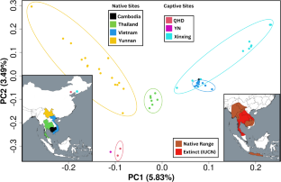
Population genetics, demographic and evolutionary history of the Dudley’s lousewort (Pedicularis dudleyi), a rare redwood forest specialist

Using genome-wide diversity and population structure to define management units in the cirio (Fouquieria columnaris), an emblematic tree of the Sonoran Desert

Whole-genome resequencing of Chinese pangolins reveals a population structure and provides insights into their conservation

Data availability.

All datasets used in this study are compiled from public repositories. The scripts and associated data from the analysis are available here: https://github.com/Ajinkya-IISERB/Pavo/tree/main/Conservation and https://doi.org/10.17632/ddwbwfjtrj.1 .

Allendorf FW, Leary RF, Spruell P, Wenburg JK (2001) The problems with hybrids: setting conservation guidelines. Trends Ecol Evol 16:613–622. https://doi.org/10.1016/S0169-5347(01)02290-X

Article   Google Scholar  

Brickle NW (2002) Habitat use, predicted distribution and conservation of green peafowl (Pavo muticus) in Dak Lak Province, Vietnam. Biol Conserv 105:189–197. https://doi.org/10.1016/S0006-3207(01)00182-3

Browning BL, Tian X, Zhou Y, Browning SR (2021) Fast two-stage phasing of large-scale sequence data. Am J Hum Genet 108:1880–1890. https://doi.org/10.1016/J.AJHG.2021.08.005

Article   CAS   PubMed   PubMed Central   Google Scholar  

Cahill JA, Soares AER, Green RE, Shapiro B (2016) Inferring species divergence times using pairwise sequential markovian coalescent modelling and low-coverage genomic data. Philos Trans R Soc B Biol Sci 371:20150138. https://doi.org/10.1098/rstb.2015.0138

Chen D, Hosner PA, Dittmann DL et al (2021) Divergence time estimation of Galliformes based on the best gene shopping scheme of ultraconserved elements. BMC Ecol Evol 21. https://doi.org/10.1186/S12862-021-01935-1

Cheng SC, Liu CB, Yao XQ et al (2023) Hologenomic insights into mammalian adaptations to myrmecophagy. Natl Sci Rev 10. https://doi.org/10.1093/NSR/NWAC174

Coates DJ, Byrne M, Moritz C (2018) Genetic diversity and conservation units: dealing with the species-population continuum in the age of genomics. Front Ecol Evol 6:165. https://doi.org/10.3389/FEVO.2018.00165/BIBTEX

Conner K, Hartl DL (2004) A primer of Ecological Genetics: a textbook. ISBN: 9780878932023

Conway W (2003) The role of zoos in the 21st century1. Int Zoo Yearb 38:7–13. https://doi.org/10.1111/J.1748-1090.2003.TB02059.X

Conway WG (2011) Buying time for wild animals with zoos. Zoo Biol 30:1–8. https://doi.org/10.1002/ZOO.20352

Article   PubMed   Google Scholar  

Darriba Di, Posada D, Kozlov AM et al (2020) ModelTest-NG: a New and Scalable Tool for the selection of DNA and protein evolutionary models. Mol Biol Evol 37:291–294. https://doi.org/10.1093/MOLBEV/MSZ189

Delacour J, Harrison JC, John C, World Pheasant Association (1977). The pheasants of the world. 395. ISBN-10 ‏: ‎0904558371

Dong F, Kuo H-CC, Chen G-LL et al (2021) Population genomic, climatic and anthropogenic evidence suggest the role of human forces in endangerment of green peafowl ( Pavo muticus ). Proc Biol Sci. 288(1948):20210073. https://doi.org/10.1098/rspb.2021.0073

Du HY, Zhang XY, Dinh TD et al (2020) Identification of hybrid green peafowl using mitochondrial and nuclear markers. Conserv Genet Resour 12:669–683. https://doi.org/10.1007/S12686-020-01159-3/TABLES/5

Ernst M, Jønsson KA, Ericson PGP et al (2022) Utilising museomics to trace the complex history and species boundaries in an avian-study system of conservation concern. Hered 2022 1283 128:159–168. https://doi.org/10.1038/s41437-022-00499-0

Espindola-Hernandez P, Mueller JC, Kempenaers B (2022) Genomic signatures of the evolution of a diurnal lifestyle in Strigiformes. G3 Genes|Genomes|Genetics 12(8):jkac135. https://doi.org/10.1093/G3JOURNAL/JKAC135

European Conservation Breeding Group (2023) PMI TN Stud book program E. In: Details regarding Studb. PMI-TN. http://pfauenfarm.de/Home-English/Our-Peafowl/Pavo-Mutisus-Imperator-E/PMI-TN-Stud-book-program-E/pmi-tn-stud-book-program-e.html . Accessed 4 May 2023

Evanno G, Regnaut S, Goudet J (2005) Detecting the number of clusters of individuals using the software STRUCTURE: a simulation study. Mol Ecol 14:2611–2620. https://doi.org/10.1111/J.1365-294X.2005.02553.X

Article   CAS   PubMed   Google Scholar  

Fraser J, Wharton D (2007) The future of Zoos: a New Model for Cultural Institutions. Curator Museum J 50:41–54. https://doi.org/10.1111/J.2151-6952.2007.TB00248.X

Funk WC, McKay JK, Hohenlohe PA, Allendorf FW (2012) Harnessing genomics for delineating conservation units. Trends Ecol Evol 27:489–496. https://doi.org/10.1016/J.TREE.2012.05.012

Article   PubMed   PubMed Central   Google Scholar  

Gautier M, Klassmann A, Vitalis R (2017) Rehh 2.0: a reimplementation of the R package rehh to detect positive selection from haplotype structure. Mol Ecol Resour 17:78–90. https://doi.org/10.1111/1755-0998.12634

Gu B, Wang F (2021) A review on the ecology and conservation biology of green peafowl (Pavo muticus). Biodivers Sci 29:1554. https://doi.org/10.17520/BIODS.2021144

Hernowo JB, Mardiastuti ANI, Alikodra HS, Kusmana CECEP (2011) Behavior Ecology of the Javan Green Peafowl (Pavo muticus muticus Linnaeus 1758) in baluran and alas Purwo National Park, East Java. HAYATI J Biosci 18:164–176. https://doi.org/10.4308/hjb.18.4.164

Höglund J, Laurila A, Rödin-Mörch P (2019) Population Genomics and Wildlife Adaptation in the Face of Climate Change. 333–355. https://doi.org/10.1007/13836_2019_69

Jackson CE (2006) Peacock. Reaktion Books, London, U.K. ISBN-10: 1861892934

Google Scholar  

Jaiswal SK, Gupta A, Saxena R et al (2018) Genome sequence of peacock reveals the Peculiar Case of a glittering bird. Front Genet 9:392. https://doi.org/10.3389/fgene.2018.00392

Johnson CN, Balmford A, Brook BW et al (2017) Biodiversity losses and conservation responses in the Anthropocene. Sci (80-) 356:270–275. https://doi.org/10.1126/SCIENCE.AAM9317/SUPPL_FILE/AAM9317_JOHNSON_SM.PDF

Article   CAS   Google Scholar  

Kardos M, Shafer ABA (2018) The peril of gene-targeted conservation. Trends Ecol Evol 33:827–839. https://doi.org/10.1016/J.TREE.2018.08.011

Kishida T (2017) Population history of Antarctic and common minke whales inferred from individual whole-genome sequences. Mar Mammal Sci 33:645–652. https://doi.org/10.1111/mms.12369

Ko S, Chu BB, Peterson D et al (2023) Unsupervised discovery of ancestry-informative markers and genetic admixture proportions in biobank-scale datasets. Am J Hum Genet 110:314–325. https://doi.org/10.1016/J.AJHG.2022.12.008

Kong D, Wu F, Shan P et al (2018) Status and distribution changes of the endangered green peafowl (Pavo muticus) in China over the past three decades (1990s-2017). Avian Res 9:1–9. https://doi.org/10.1186/S40657-018-0110-0/TABLES/3

Kopelman NM, Mayzel J, Jakobsson M et al (2015) Clumpak: a program for identifying clustering modes and packaging population structure inferences across K. Mol Ecol Resour 15:1179–1191. https://doi.org/10.1111/1755-0998.12387

Korneliussen TS, Albrechtsen A, Nielsen R (2014) ANGSD: analysis of next generation sequencing data. BMC Bioinformatics 15:356.  https://doi.org/10.1186/s12859-014-0356-4

Korunes KL, Samuk K (2021) Pixy: unbiased estimation of nucleotide diversity and divergence in the presence of missing data. Mol Ecol Resour 21:1359–1368. https://doi.org/10.1111/1755-0998.13326

Kozlov AM, Darriba D, Flouri T et al (2019) RAxML-NG: a fast, scalable and user-friendly tool for maximum likelihood phylogenetic inference. Bioinformatics 35:4453–4455. https://doi.org/10.1093/BIOINFORMATICS/BTZ305

Kozma R, Melsted P, Magnússon KP, Höglund J (2016) Looking into the past – the reaction of three grouse species to climate change over the last million years using whole genome sequences. Mol Ecol 25:570–580. https://doi.org/10.1111/MEC.13496

Lee TH, Guo H, Wang X et al (2014) SNPhylo: a pipeline to construct a phylogenetic tree from huge SNP data. BMC Genomics 15:162. https://doi.org/10.1186/1471-2164-15-162

Li H (2013) Aligning sequence reads, clone sequences and assembly contigs with BWA-MEM. arxiv. https://doi.org/10.48550/arXiv.1303.3997

Li H, Barrett J (2011) A statistical framework for SNP calling, mutation discovery, association mapping and population genetical parameter estimation from sequencing data. Bioinformatics 27:2987–2993. https://doi.org/10.1093/BIOINFORMATICS/BTR509

Li H, Durbin R (2011) Inference of human population history from individual whole-genome sequences. Nature 475:493–496. https://doi.org/10.1038/nature10231

Li H, Handsaker B, Wysoker A et al (2009) The sequence Alignment/Map format and SAMtools. Bioinformatics 25:2078–2079. https://doi.org/10.1093/bioinformatics/btp352

Lin F (2010) A Monograph of Peafowl of the Genus Pavo. Can be accessed at https://github.com/Ajinkya-IISERB/Pavo/blob/main/Conservation/A-monograph-of-peafowl-of-the-genus-pavo-by-frank-lin-photo.pdf

Mason N, Ward M, Watson JEM et al (2020) Global opportunities and challenges for transboundary conservation. Nat Ecol Evol 2020 45 4:694–701. https://doi.org/10.1038/s41559-020-1160-3

McGowan PJK, Duckworth JW, Xianji W et al (1998) A review of the status of the Green Peafowl Pavo muticus and recommendations for future action. Bird Conserv Int 8:331–348. https://doi.org/10.1017/S0959270900002100

Meisner J, Albrechtsen A (2018) Inferring Population structure and admixture proportions in low-depth NGS data. Genetics 210:719–731. https://doi.org/10.1534/GENETICS.118.301336

Mikkelson GM, Gonzalez A, Peterson GD (2007) Economic Inequality predicts Biodiversity loss. PLoS ONE 2:e444. https://doi.org/10.1371/JOURNAL.PONE.0000444

Nuttall M, Nut M, Ung V, O’Kelly H (2017) Abundance estimates for the endangered green peafowl Pavo muticus in Cambodia: identification of a globally important site for conservation. Bird Conserv Int 27:127–139. https://doi.org/10.1017/S0959270916000083

Palsbøll PJ, Bérubé M, Allendorf FW (2007) Identification of management units using population genetic data. Trends Ecol Evol 22:11–16. https://doi.org/10.1016/J.TREE.2006.09.003

Raj A, Stephens M, Pritchard JK (2014) FastSTRUCTURE: variational inference of population structure in large SNP data sets. Genetics 197:573–589. https://doi.org/10.1534/GENETICS.114.164350/-/DC1

Rellstab C, Dauphin B, Exposito-Alonso M (2021) Prospects and limitations of genomic offset in conservation management. Evol Appl 14:1202–1212. https://doi.org/10.1111/EVA.13205

Salles T, Mallard C, Husson L et al (2021) Quaternary landscape dynamics boosted species dispersal across Southeast Asia. Commun Earth Environ 2021 21 2:1–12. https://doi.org/10.1038/s43247-021-00311-7

Saridnirun G, Sukumal N, Grainger MJ, Savini T (2021) Living with human encroachment: Status and distribution of Green Peafowl in northern stronghold of Thailand. Glob Ecol Conserv 28:e01674. https://doi.org/10.1016/J.GECCO.2021.E01674

Segelbacher G, Bosse M, Burger P et al (2021) New developments in the field of genomic technologies and their relevance to conservation management. Conserv Genet 2021 232 23:217–242. https://doi.org/10.1007/S10592-021-01415-5

Sih A, Jonsson BG, Luikart G (2000) Habitat loss: ecological, evolutionary and genetic consequences. Trends Ecol Evol 15:132–134. https://doi.org/10.1016/S0169-5347(99)01799-1

Skotte L, Korneliussen TS, Albrechtsen A (2013) Estimating individual admixture proportions from next generation sequencing data. Genetics 195:693–702. https://doi.org/10.1534/GENETICS.113.154138

Sodhi NS, Koh LP, Brook BW, Ng PKL (2004) Southeast asian biodiversity: an impending disaster. Trends Ecol Evol 19:654–660. https://doi.org/10.1016/J.TREE.2004.09.006

Song S, Sliwerska E, Emery S, Kidd JM (2017) Modeling human population separation history using physically phased genomes. Genetics 205:385–395. https://doi.org/10.1534/genetics.116.192963

Song K, Gao B, Halvarsson P et al (2020) Genomic analysis of demographic history and ecological niche modeling in the endangered chinese Grouse Tetrastes sewerzowi. BMC Genomics 21:1–9. https://doi.org/10.1186/S12864-020-06957-5/FIGURES/4

Sukumal N, McGowan PJK, Savini T (2015) Change in status of green peafowl Pavo muticus (Family Phasianidae) in Southcentral Vietnam: a comparison over 15 years. Glob Ecol Conserv 3:11–19. https://doi.org/10.1016/J.GECCO.2014.10.007

Sukumal N, Dowell SD, Savini T (2017) Micro-habitat selection and population recovery of the Endangered Green Peafowl Pavo muticus in western Thailand: implications for conservation guidance. Bird Conserv Int 27:414–430. https://doi.org/10.1017/S095927091600037X

Sukumal N, Dowell SD, Savini T (2020) Modelling occurrence probability of the endangered green peafowl Pavo muticus in mainland Southeast Asia: applications for landscape conservation and management. Oryx 54:30–39. https://doi.org/10.1017/S003060531900005X

Talla V, Mrazek V, Höglund J, Backström N (2023) Whole genome re-sequencing uncovers significant population structure and low genetic diversity in the endangered clouded apollo (Parnasssius mnemosyne) in Sweden. Conserv Genet 1:1–10. https://doi.org/10.1007/S10592-023-01502-9/FIGURES/4

Teerlink CC, Jurynec MJ, Hernandez R et al (2021) A role for the MEGF6 gene in predisposition to osteoporosis. Ann Hum Genet 85:58–72. https://doi.org/10.1111/AHG.12408

van Balen S, Prawiradilaga DM, Indrawan M (1995) The distribution and status of green peafowl Pavo muticus in Java. Biol Conserv 71:289–297. https://doi.org/10.1016/0006-3207(94)00048-U

Voris HK (2000) Maps of Pleistocene sea levels in Southeast Asia: shorelines, river systems and time durations. J Biogeogr 27:1153–1167. https://doi.org/10.1046/J.1365-2699.2000.00489.X

Wharton D (2008) The future of zoo biology. Zoo Biol 27:498–504. https://doi.org/10.1002/ZOO.20204

Wolf JBW, Ellegren H (2017) Making sense of genomic islands of differentiation in light of speciation. Nat Rev Genet 18:87–100. https://doi.org/10.1038/nrg.2016.133

Woodruff DS (2010) Biogeography and conservation in Southeast Asia: how 2.7 million years of repeated environmental fluctuations affect today’s patterns and the future of the remaining refugial-phase biodiversity. Biodivers Conserv 19:919–941. https://doi.org/10.1007/S10531-010-9783-3/FIGURES/3

Wright AE, Harrison PW, Zimmer F et al (2015) Variation in promiscuity and sexual selection drives avian rate of Faster-Z evolution. Mol Ecol 24:1218–1235. https://doi.org/10.1111/MEC.13113

Wright BR, Farquharson KA, McLennan EA et al (2020) A demonstration of conservation genomics for threatened species management. Mol Ecol Resour 20:1526–1541. https://doi.org/10.1111/1755-0998.13211

Zhang X, Lin C, Li H et al (2022) Chromosome-Level Genome Assembly of the Green Peafowl (Pavo muticus). Genome Biol Evol 14. https://doi.org/10.1093/GBE/EVAC015

Zhou H, Sinsheimer JS, Bates DM et al (2020) OpenMendel: a Cooperative Programming Project for Statistical Genetics. Hum Genet 139:61. https://doi.org/10.1007/S00439-019-02001-Z

Download references

Acknowledgements

We want to thank Kermit Blackwood for the extensive discussion regarding the morphological diversity associated with different landscapes within green peafowl. We want to thank the two anonymous reviewers from the first round of peer review for their insightful comments regarding the writing and additional analysis that immensely helped improve the manuscript. The two new anonymous reviewers in the second round of peer review provided critical new perspectives and further enhanced the quality of the manuscript. We thank the Ministry of Human Resource Development for awarding a fellowship to ABP. The Department of Biotechnology, Ministry of Science and Technology, India (Grant no. BT/11/IYBA/2018/03) and Science and Engineering Research Board (Grant no. ECR/2017/001430) provided computational resources (i.e., Har Gobind Khorana Computational Biology cluster).

Author information

Authors and affiliations.

Academic Building III, Computational Evolutionary Genomics Lab, Department of Biological Sciences, IISER Bhopal, Indore By-pass Road Bhauri Bhopal, 462066, Bhopal, Madhya Pradesh, India

Ajinkya Bharatraj Patil & Nagarjun Vijay

You can also search for this author in PubMed   Google Scholar

Contributions

ABP analyzed the genomic data and generated all the results. ABP wrote the manuscript with inputs from NV.

Corresponding author

Correspondence to Nagarjun Vijay .

Ethics declarations

Competing interests.

The authors declare no competing interests.

Additional information

Publisher’s note.

Springer Nature remains neutral with regard to jurisdictional claims in published maps and institutional affiliations.

Electronic supplementary material

Below is the link to the electronic supplementary material.

Supplementary Material 1

Supplementary material 2, supplementary material 3, supplementary material 4, supplementary material 5, rights and permissions.

Springer Nature or its licensor (e.g. a society or other partner) holds exclusive rights to this article under a publishing agreement with the author(s) or other rightsholder(s); author self-archiving of the accepted manuscript version of this article is solely governed by the terms of such publishing agreement and applicable law.

Reprints and permissions

About this article

Patil, A.B., Vijay, N. Conservation implications of diverse demographic histories: the case study of green peafowl ( Pavo muticus , Linnaeus 1766). Conserv Genet 25 , 455–468 (2024). https://doi.org/10.1007/s10592-023-01580-9

Download citation

Received : 12 May 2023

Accepted : 23 September 2023

Published : 14 October 2023

Issue Date : April 2024

DOI : https://doi.org/10.1007/s10592-023-01580-9

Share this article

Anyone you share the following link with will be able to read this content:

Sorry, a shareable link is not currently available for this article.

Provided by the Springer Nature SharedIt content-sharing initiative

• Conservation
• Demographic history
• Endangered species
• Evolutionarily significant units (ESUs)
• Green peafowl
• Population structure
• Find a journal
• Publish with us
• Track your research

Thank you for visiting nature.com. You are using a browser version with limited support for CSS. To obtain the best experience, we recommend you use a more up to date browser (or turn off compatibility mode in Internet Explorer). In the meantime, to ensure continued support, we are displaying the site without styles and JavaScript.

• View all journals
• Explore content
• About the journal
• Publish with us
• Sign up for alerts
• Published: 06 September 2017

Massive genetic study shows how humans are evolving

• Bruno Martin  

Nature ( 2017 ) Cite this article

8561 Accesses

2 Citations

877 Altmetric

Metrics details

Analysis of 215,000 people's DNA suggests variants that shorten life are being selected against.

A huge genetic study that sought to pinpoint how the human genome is evolving suggests that natural selection is getting rid of harmful genetic mutations that shorten people’s lives. The work, published in PLoS Biology 1 , analysed DNA from 215,000 people and is one of the first attempts to probe directly how humans are evolving over one or two generations.

To identify which bits of the human genome might be evolving, researchers scoured large US and UK genetic databases for mutations whose prevalence changed across different age groups. For each person, the parents’ age of death was recorded as a measure of longevity, or their own age in some cases.

“If a genetic variant influences survival, its frequency should change with the age of the surviving individuals,” says Hakhamanesh Mostafavi, an evolutionary biologist at Columbia University in New York City who led the study. People who carry a harmful genetic variant die at a higher rate, so the variant becomes rarer in the older portion of the population.

Mostafavi and his colleagues tested more than 8 million common mutations, and found two that seemed to become less prevalent with age. A variant of the APOE gene, which is strongly linked to Alzheimer’s disease, was rarely found in women over 70. And a mutation in the CHRNA3 gene associated with heavy smoking in men petered out in the population starting in middle age. People without these mutations have a survival edge and are more likely to live longer, the researchers suggest.

This is not, by itself, evidence of evolution at work. In evolutionary terms, having a long life isn’t as important as having a reproductively fruitful one, with many children who survive into adulthood and birth their own offspring. So harmful mutations that exert their effects after reproductive age could be expected to be ‘neutral’ in the eyes of evolution, and not selected against.

But if that were the case, there would be plenty of such mutations still kicking around in the genome, the authors argue. That such a large study found only two strongly suggests that evolution is “weeding” them out, says Mostafavi, and that others have probably already been purged from the population by natural selection.

Links to longevity

Why these late-acting mutations might lower a person’s genetic fitness — their ability to reproduce and spread their genes — remains an open question.

The authors suggest that for men, it could be that those who live longer can have more children, but this is unlikely to be the whole story. So scientists are considering two other explanations for why longevity is important. First, parents surviving into old age in good health can care for their children and grandchildren, increasing the later generations’ chances of surviving and reproducing. This is sometimes known as the ‘grandmother hypothesis’, and may explain why humans tend to live long after menopause.

Second, it’s possible that genetic variants that are explicitly bad in old age are also harmful — but more subtly — earlier in life. “You would need extremely large samples to see these small effects,” says Iain Mathieson, a population geneticist at the University of Pennsylvania in Philadelphia, so that’s why it’s not yet possible to tell whether this is the case.

The researchers also found that certain groups of genetic mutations, which individually would not have a measurable effect but together accounted for health threats, appeared less often in people who were expected to have long lifespans than in those who weren't. These included predispositions to asthma, high body mass index and high cholesterol. Most surprising, however, was the finding that sets of mutations that delay puberty and childbearing are more prevalent in long-lived people.

To see a genetic link to delayed childbearing is intriguing, says Jonathan Pritchard, a geneticist at Stanford University in California. The link between longevity and late fertility has been spotted before, but those studies could not discount the effects of wealth and education, because people with high levels of both tend to have children later in life. The latest genetic evidence makes Pritchard think there is an evolutionary trade-off between fertility and longevity, which had previously been studied only in other animals. “To actually find this in humans is really pretty cool,” he says. “I think it's a really nice study.”

Studying ongoing evolution in humans is notoriously difficult. Scientists who want to observe selection directly would need to measure the frequency of a mutation in one generation, and then again in all that generation’s children and, better still, grandchildren, says Gil McVean, a statistical geneticist at the University of Oxford, UK. “That would be very hard to do well,” he says. “You would need vast samples”.

Mostafavi, H. et al. PLoS Biol. 15 , e2002458 (2017).

Article   Google Scholar  

Download references

You can also search for this author in PubMed   Google Scholar

Related links

Related links in nature research.

Scientists track last 2,000 years of British evolution 2016-May-17

Gene variants linked to success at school prove divisive 2016-May-11

Genetic secrets of the healthy elderly unveiled 2016-Apr-21

Studies slow the human DNA clock 2012-Sep-18

Rights and permissions

Reprints and permissions

About this article

Cite this article.

Martin, B. Massive genetic study shows how humans are evolving. Nature (2017). https://doi.org/10.1038/nature.2017.22565

Download citation

Published : 06 September 2017

DOI : https://doi.org/10.1038/nature.2017.22565

Share this article

Anyone you share the following link with will be able to read this content:

Sorry, a shareable link is not currently available for this article.

Provided by the Springer Nature SharedIt content-sharing initiative

Quick links

• Explore articles by subject
• Guide to authors
• Editorial policies

Sign up for the Nature Briefing: Translational Research newsletter — top stories in biotechnology, drug discovery and pharma.

File(s) stored somewhere else

Please note: Linked content is NOT stored on Ag Data Commons and we can ' t guarantee its availability, quality, security or accept any liability.

Data from: Estimation of genetic parameters and their sampling variances for quantitative traits in the type 2 modified augmented design

The type 2 modified augmented design (MAD2) is an efficient unreplicated experimental design used for evaluating large numbers of lines in plant breeding and for assessing genetic variation in a population. Statistical methods and data adjustment for soil heterogeneity have been previously described for this design. In the absence of replicated test genotypes in MAD2, their total variance cannot be partitioned into genetic and error components as required to estimate heritability and genetic correlation of quantitative traits, the two conventional genetic parameters used for breeding selection. We propose a method of estimating the error variance of unreplicated genotypes that uses replicated controls, and then of estimating the genetic parameters. Using the Delta method, we also derived formulas for estimating the sampling variances of the genetic parameters. Computer simulations indicated that the proposed method for estimating genetic parameters and their sampling variances was feasible and the reliability of the estimates was positively associated with the level of heritability of the trait. A case study of estimating the genetic parameters of three quantitative traits, iodine value, oil content, and linolenic acid content, in a biparental recombinant inbred line population of flax with 243 individuals, was conducted using our statistical models. A joint analysis of data over multiple years and sites was suggested for genetic parameter estimation. A pipeline module using SAS and Perl was developed to facilitate data analysis and appended to the previously developed MAD data analysis pipeline ( http://probes.pw.usda.gov/bioinformatics_tools/MADPipeline/index.html ).

Resource Title: Table S1. The raw phenotypic data of a population with 243 RILs derived from a cross between ‘CDC Bethune’ and ‘Macbeth’ (BM) for the case study..

File Name: 1-s2.0-S2214514116000179-mmc1.xlsx, url: https://ars.els-cdn.com/content/image/1-s2.0-S2214514116000179-mmc1.xlsx

Supplementary data

Agriculture and Agri-Food Canada

Genome canada, western grains research foundation, data contact name, data contact email.

• Not specified

ISO Topic Category

National agricultural library thesaurus terms, primary article pubag handle.

• https://pubag.nal.usda.gov/catalog/5280945

Pending citation

Public access level, preferred dataset citation, usage metrics.

• Genetics not elsewhere classified