hypothesis test spss

University Library

SPSS Tutorial: General Statistics and Hypothesis Testing

• About This Tutorial
• SPSS Components
• Importing Data
• General Statistics and Hypothesis Testing
• Further Resources

Merging Files based on a shared variable.

This section and the "Graphics" section provide a quick tutorial for a few common functions in SPSS, primarily to provide the reader with a feel for the SPSS user interface. This is not a comprehensive tutorial, but SPSS itself provides comprehensive tutorials and case studies through it's help menu. SPSS's help menu is more than a quick reference. It provides detailed information on how and when to use SPSS's various menu options. See the "Further Resources" section for more information. 

To perform a one sample t-test click "Analyze"→"Compare Means"→"One Sample T-Test" and the following dialog box will appear:

The dialogue allows selection of any scale variable from the box at the left and a test value that represents a hypothetical mean. Select the test variable and set the test value, then press "Ok." Three tables will appear in the Output Viewer:

The first table gives descriptive statistics about the variable. The second shows the results of the t_test, including the "t" statistic, the degrees of freedom ("df") the p-value ("Sig."), the difference of the test value from the variable mean, and the upper and lower bounds for a ninety-five percent confidence interval. The final table shows one-sample effect sizes.

One-Way ANOVA

In the Data Editor, select "Analyze"→"Compare Means"→"One-Way ANOVA..." to open the dialog box shown below.

To generate the ANOVA statistic the variables chosen cannot have a "Nominal" level of measurement; they must be "ordinal." 

Once the nominal variables have been changed to ordinal, select "the dependent variable and  the factor, then click "OK." The following output will appear in the Output Viewer:

Linear Regression

To obtain a linear regression select "Analyze"->"Regression"->"Linear" from the menu, calling up the dialog box shown below:

The output of this most basic case produces a summary chart showing R, R-square, and the Standard error of the prediction; an ANOVA chart; and a chart providing statistics on model coefficients:

For Multiple regression, simply add more independent variables in the "Linear Regression" dialogue box. To plot a regression line see the "Legacy Dialogues" section of the "Graphics" tab.

Scholarly Commons

• << Previous: Importing Data
• Next: Graphics >>
• Last Updated: Jul 9, 2024 5:55 PM
• URL: https://guides.library.illinois.edu/spss

• Skip to secondary menu
• Skip to main content
• Skip to primary sidebar

Statistics By Jim

Making statistics intuitive

One-Tailed and Two-Tailed Hypothesis Tests Explained

By Jim Frost 60 Comments

Choosing whether to perform a one-tailed or a two-tailed hypothesis test is one of the methodology decisions you might need to make for your statistical analysis. This choice can have critical implications for the types of effects it can detect, the statistical power of the test, and potential errors.

In this post, you’ll learn about the differences between one-tailed and two-tailed hypothesis tests and their advantages and disadvantages. I include examples of both types of statistical tests. In my next post, I cover the decision between one and two-tailed tests in more detail.

What Are Tails in a Hypothesis Test?

First, we need to cover some background material to understand the tails in a test. Typically, hypothesis tests take all of the sample data and convert it to a single value, which is known as a test statistic. You’re probably already familiar with some test statistics. For example, t-tests calculate t-values . F-tests, such as ANOVA, generate F-values . The chi-square test of independence and some distribution tests produce chi-square values. All of these values are test statistics. For more information, read my post about Test Statistics .

These test statistics follow a sampling distribution. Probability distribution plots display the probabilities of obtaining test statistic values when the null hypothesis is correct. On a probability distribution plot, the portion of the shaded area under the curve represents the probability that a value will fall within that range.

The graph below displays a sampling distribution for t-values. The two shaded regions cover the two-tails of the distribution.

Keep in mind that this t-distribution assumes that the null hypothesis is correct for the population. Consequently, the peak (most likely value) of the distribution occurs at t=0, which represents the null hypothesis in a t-test. Typically, the null hypothesis states that there is no effect. As t-values move further away from zero, it represents larger effect sizes. When the null hypothesis is true for the population, obtaining samples that exhibit a large apparent effect becomes less likely, which is why the probabilities taper off for t-values further from zero.

Related posts : How t-Tests Work and Understanding Probability Distributions

Critical Regions in a Hypothesis Test

In hypothesis tests, critical regions are ranges of the distributions where the values represent statistically significant results. Analysts define the size and location of the critical regions by specifying both the significance level (alpha) and whether the test is one-tailed or two-tailed.

Consider the following two facts:

• The significance level is the probability of rejecting a null hypothesis that is correct.
• The sampling distribution for a test statistic assumes that the null hypothesis is correct.

Consequently, to represent the critical regions on the distribution for a test statistic, you merely shade the appropriate percentage of the distribution. For the common significance level of 0.05, you shade 5% of the distribution.

Related posts : Significance Levels and P-values and T-Distribution Table of Critical Values

Two-Tailed Hypothesis Tests

Two-tailed hypothesis tests are also known as nondirectional and two-sided tests because you can test for effects in both directions. When you perform a two-tailed test, you split the significance level percentage between both tails of the distribution. In the example below, I use an alpha of 5% and the distribution has two shaded regions of 2.5% (2 * 2.5% = 5%).

When a test statistic falls in either critical region, your sample data are sufficiently incompatible with the null hypothesis that you can reject it for the population.

In a two-tailed test, the generic null and alternative hypotheses are the following:

• Null : The effect equals zero.
• Alternative :  The effect does not equal zero.

The specifics of the hypotheses depend on the type of test you perform because you might be assessing means, proportions, or rates.

Example of a two-tailed 1-sample t-test

Suppose we perform a two-sided 1-sample t-test where we compare the mean strength (4.1) of parts from a supplier to a target value (5). We use a two-tailed test because we care whether the mean is greater than or less than the target value.

To interpret the results, simply compare the p-value to your significance level. If the p-value is less than the significance level, you know that the test statistic fell into one of the critical regions, but which one? Just look at the estimated effect. In the output below, the t-value is negative, so we know that the test statistic fell in the critical region in the left tail of the distribution, indicating the mean is less than the target value. Now we know this difference is statistically significant.

We can conclude that the population mean for part strength is less than the target value. However, the test had the capacity to detect a positive difference as well. You can also assess the confidence interval. With a two-tailed hypothesis test, you’ll obtain a two-sided confidence interval. The confidence interval tells us that the population mean is likely to fall between 3.372 and 4.828. This range excludes the target value (5), which is another indicator of significance.

Advantages of two-tailed hypothesis tests

You can detect both positive and negative effects. Two-tailed tests are standard in scientific research where discovering any type of effect is usually of interest to researchers.

One-Tailed Hypothesis Tests

One-tailed hypothesis tests are also known as directional and one-sided tests because you can test for effects in only one direction. When you perform a one-tailed test, the entire significance level percentage goes into the extreme end of one tail of the distribution.

In the examples below, I use an alpha of 5%. Each distribution has one shaded region of 5%. When you perform a one-tailed test, you must determine whether the critical region is in the left tail or the right tail. The test can detect an effect only in the direction that has the critical region. It has absolutely no capacity to detect an effect in the other direction.

In a one-tailed test, you have two options for the null and alternative hypotheses, which corresponds to where you place the critical region.

You can choose either of the following sets of generic hypotheses:

• Null : The effect is less than or equal to zero.
• Alternative : The effect is greater than zero.

• Null : The effect is greater than or equal to zero.
• Alternative : The effect is less than zero.

Again, the specifics of the hypotheses depend on the type of test you perform.

Notice how for both possible null hypotheses the tests can’t distinguish between zero and an effect in a particular direction. For example, in the example directly above, the null combines “the effect is greater than or equal to zero” into a single category. That test can’t differentiate between zero and greater than zero.

Example of a one-tailed 1-sample t-test

Suppose we perform a one-tailed 1-sample t-test. We’ll use a similar scenario as before where we compare the mean strength of parts from a supplier (102) to a target value (100). Imagine that we are considering a new parts supplier. We will use them only if the mean strength of their parts is greater than our target value. There is no need for us to differentiate between whether their parts are equally strong or less strong than the target value—either way we’d just stick with our current supplier.

Consequently, we’ll choose the alternative hypothesis that states the mean difference is greater than zero (Population mean – Target value > 0). The null hypothesis states that the difference between the population mean and target value is less than or equal to zero.

To interpret the results, compare the p-value to your significance level. If the p-value is less than the significance level, you know that the test statistic fell into the critical region. For this study, the statistically significant result supports the notion that the population mean is greater than the target value of 100.

Confidence intervals for a one-tailed test are similarly one-sided. You’ll obtain either an upper bound or a lower bound. In this case, we get a lower bound, which indicates that the population mean is likely to be greater than or equal to 100.631. There is no upper limit to this range.

A lower-bound matches our goal of determining whether the new parts are stronger than our target value. The fact that the lower bound (100.631) is higher than the target value (100) indicates that these results are statistically significant.

This test is unable to detect a negative difference even when the sample mean represents a very negative effect.

Advantages and disadvantages of one-tailed hypothesis tests

One-tailed tests have more statistical power to detect an effect in one direction than a two-tailed test with the same design and significance level. One-tailed tests occur most frequently for studies where one of the following is true:

• Effects can exist in only one direction.
• Effects can exist in both directions but the researchers only care about an effect in one direction. There is no drawback to failing to detect an effect in the other direction. (Not recommended.)

The disadvantage of one-tailed tests is that they have no statistical power to detect an effect in the other direction.

As part of your pre-study planning process, determine whether you’ll use the one- or two-tailed version of a hypothesis test. To learn more about this planning process, read 5 Steps for Conducting Scientific Studies with Statistical Analyses .

This post explains the differences between one-tailed and two-tailed statistical hypothesis tests. How these forms of hypothesis tests function is clear and based on mathematics. However, there is some debate about when you can use one-tailed tests. My next post explores this decision in much more depth and explains the different schools of thought and my opinion on the matter— When Can I Use One-Tailed Hypothesis Tests .

If you’re learning about hypothesis testing and like the approach I use in my blog, check out my Hypothesis Testing book! You can find it at Amazon and other retailers.

Share this:

Reader Interactions

June 26, 2022 at 12:14 pm

Hi, Can help me with figuring out the null and alternative hypothesis of the following statement? Some claimed that the real average expenditure on beverage by general people is at least $10.

February 19, 2022 at 6:02 am

thank you for the thoroughly explanation, I’m still strugling to wrap my mind around the t-table and the relation between the alpha values for one or two tail probability and the confidence levels on the bottom (I’m understanding it so wrongly that for me it should be the oposite, like one tail 0,05 should correspond 95% CI and two tailed 0,025 should correspond to 95% because then you got the 2,5% on each side). In my mind if I picture the one tail diagram with an alpha of 0,05 I see the rest 95% inside the diagram, but for a one tail I only see 90% CI paired with a 5% alpha… where did the other 5% go? I tried to understand when you said we should just double the alpha for a one tail probability in order to find the CI but I still cant picture it. I have been trying to understand this. Like if you only have one tail and there is 0,05, shouldn’t the rest be on the other side? why is it then 90%… I know I’m missing a point and I can’t figure it out and it’s so frustrating…

February 23, 2022 at 10:01 pm

The alpha is the total shaded area. So, if the alpha = 0.05, you know that 5% of the distribution is shaded. The number of tails tells you how to divide the shaded areas. Is it all in one region (1-tailed) or do you split the shaded regions in two (2-tailed)?

So, for a one-tailed test with an alpha of 0.05, the 5% shading is all in one tail. If alpha = 0.10, then it’s 10% on one side. If it’s two-tailed, then you need to split that 10% into two–5% in both tails. Hence, the 5% in a one-tailed test is the same as a two-tailed test with an alpha of 0.10 because that test has the same 5% on one side (but there’s another 5% in the other tail).

It’s similar for CIs. However, for CIs, you shade the middle rather than the extremities. I write about that in one my articles about hypothesis testing and confidence intervals .

I’m not sure if I’m answering your question or not.

February 17, 2022 at 1:46 pm

I ran a post hoc Dunnett’s test alpha=0.05 after a significant Anova test in Proc Mixed using SAS. I want to determine if the means for treatment (t1, t2, t3) is significantly less than the means for control (p=pathogen). The code for the dunnett’s test is – LSmeans trt / diff=controll (‘P’) adjust=dunnett CL plot=control; I think the lower bound one tailed test is the correct test to run but I’m not 100% sure. I’m finding conflicting information online. In the output table for the dunnett’s test the mean difference between the control and the treatments is t1=9.8, t2=64.2, and t3=56.5. The control mean estimate is 90.5. The adjusted p-value by treatment is t1(p=0.5734), t2 (p=.0154) and t3(p=.0245). The adjusted lower bound confidence limit in order from t1-t3 is -38.8, 13.4, and 7.9. The adjusted upper bound for all test is infinity. The graphical output for the dunnett’s test in SAS is difficult to understand for those of us who are beginner SAS users. All treatments appear as a vertical line below the the horizontal line for control at 90.5 with t2 and t3 in the shaded area. For treatment 1 the shaded area is above the line for control. Looking at just the output table I would say that t2 and t3 are significantly lower than the control. I guess I would like to know if my interpretation of the outputs is correct that treatments 2 and 3 are statistically significantly lower than the control? Should I have used an upper bound one tailed test instead?

November 10, 2021 at 1:00 am

Thanks Jim. Please help me understand how a two tailed testing can be used to minimize errors in research

July 1, 2021 at 9:19 am

Hi Jim, Thanks for posting such a thorough and well-written explanation. It was extremely useful to clear up some doubts.

May 7, 2021 at 4:27 pm

Hi Jim, I followed your instructions for the Excel add-in. Thank you. I am very new to statistics and sort of enjoy it as I enter week number two in my class. I am to select if three scenarios call for a one or two-tailed test is required and why. The problem is stated:

30% of mole biopsies are unnecessary. Last month at his clinic, 210 out of 634 had benign biopsy results. Is there enough evidence to reject the dermatologist’s claim?

Part two, the wording changes to “more than of 30% of biopsies,” and part three, the wording changes to “less than 30% of biopsies…”

I am not asking for the problem to be solved for me, but I cannot seem to find direction needed. I know the elements i am dealing with are =30%, greater than 30%, and less than 30%. 210 and 634. I just don’t know what to with the information. I can’t seem to find an example of a similar problem to work with.

May 9, 2021 at 9:22 pm

As I detail in this post, a two-tailed test tells you whether an effect exists in either direction. Or, is it different from the null value in either direction. For the first example, the wording suggests you’d need a two-tailed test to determine whether the population proportion is ≠ 30%. Whenever you just need to know ≠, it suggests a two-tailed test because you’re covering both directions.

For part two, because it’s in one direction (greater than), you need a one-tailed test. Same for part three but it’s less than. Look in this blog post to see how you’d construct the null and alternative hypotheses for these cases. Note that you’re working with a proportion rather than the mean, but the principles are the same! Just plug your scenario and the concept of proportion into the wording I use for the hypotheses.

I hope that helps!

April 11, 2021 at 9:30 am

Hello Jim, great website! I am using a statistics program (SPSS) that does NOT compute one-tailed t-tests. I am trying to compare two independent groups and have justifiable reasons why I only care about one direction. Can I do the following? Use SPSS for two-tailed tests to calculate the t & p values. Then report the p-value as p/2 when it is in the predicted direction (e.g , SPSS says p = .04, so I report p = .02), and report the p-value as 1 – (p/2) when it is in the opposite direction (e.g., SPSS says p = .04, so I report p = .98)? If that is incorrect, what do you suggest (hopefully besides changing statistics programs)? Also, if I want to report confidence intervals, I realize that I would only have an upper or lower bound, but can I use the CI’s from SPSS to compute that? Thank you very much!

April 11, 2021 at 5:42 pm

Yes, for p-values, that’s absolutely correct for both cases.

For confidence intervals, if you take one endpoint of a two-side CI, it becomes a one-side bound with half the confidence level.

Consequently, to obtain a one-sided bound with your desired confidence level, you need to take your desired significance level (e.g., 0.05) and double it. Then subtract it from 1. So, if you’re using a significance level of 0.05, double that to 0.10 and then subtract from 1 (1 – 0.10 = 0.90). 90% is the confidence level you want to use for a two-sided test. After obtaining the two-sided CI, use one of the endpoints depending on the direction of your hypothesis (i.e., upper or lower bound). That’s produces the one-sided the bound with the confidence level that you want. For our example, we calculated a 95% one-sided bound.

March 3, 2021 at 8:27 am

Hi Jim. I used the one-tailed(right) statistical test to determine an anomaly in the below problem statement: On a daily basis, I calculate the (mapped_%) in a common field between two tables.

The way I used the t-test is: On any particular day, I calculate the sample_mean, S.D and sample_count (n=30) for the last 30 days including the current day. My null hypothesis, H0 (pop. mean)=95 and H1>95 (alternate hypothesis). So, I calculate the t-stat based on the sample_mean, pop.mean, sample S.D and n. I then choose the t-crit value for 0.05 from my t-ditribution table for dof(n-1). On the current day if my abs.(t-stat)>t-crit, then I reject the null hypothesis and I say the mapped_pct on that day has passed the t-test.

I get some weird results here, where if my mapped_pct is as low as 6%-8% in all the past 30 days, the t-test still gets a “pass” result. Could you help on this? If my hypothesis needs to be changed.

I would basically look for the mapped_pct >95, if it worked on a static trigger. How can I use the t-test effectively in this problem statement?

December 18, 2020 at 8:23 pm

Hello Dr. Jim, I am wondering if there is evidence in one of your books or other source you could provide, which supports that it is OK not to divide alpha level by 2 in one-tailed hypotheses. I need the source for supporting evidence in a Portfolio exercise and couldn’t find one.

I am grateful for your reply and for your statistics knowledge sharing!

November 27, 2020 at 10:31 pm

If I did a one directional F test ANOVA(one tail ) and wanted to calculate a confidence interval for each individual groups (3) mean . Would I use a one tailed or two tailed t , within my confidence interval .

November 29, 2020 at 2:36 am

Hi Bashiru,

F-tests for ANOVA will always be one-tailed for the reasons I discuss in this post. To learn more about, read my post about F-tests in ANOVA .

For the differences between my groups, I would not use t-tests because the family-wise error rate quickly grows out of hand. To learn more about how to compare group means while controlling the familywise error rate, read my post about using post hoc tests with ANOVA . Typically, these are two-side intervals but you’d be able to use one-sided.

November 26, 2020 at 10:51 am

Hi Jim, I had a question about the formulation of the hypotheses. When you want to test if a beta = 1 or a beta = 0. What will be the null hypotheses? I’m having trouble with finding out. Because in most cases beta = 0 is the null hypotheses but in this case you want to test if beta = 0. so i’m having my doubts can it in this case be the alternative hypotheses or is it still the null hypotheses?

Kind regards, Noa

November 27, 2020 at 1:21 am

Typically, the null hypothesis represents no effect or no relationship. As an analyst, you’re hoping that your data have enough evidence to reject the null and favor the alternative.

Assuming you’re referring to beta as in regression coefficients, zero represents no relationship. Consequently, beta = 0 is the null hypothesis.

You might hope that beta = 1, but you don’t usually include that in your alternative hypotheses. The alternative hypothesis usually states that it does not equal no effect. In other words, there is an effect but it doesn’t state what it is.

There are some exceptions to the above but I’m writing about the standard case.

November 22, 2020 at 8:46 am

Your articles are a help to intro to econometrics students. Keep up the good work! More power to you!

November 6, 2020 at 11:25 pm

Hello Jim. Can you help me with these please?

Write the null and alternative hypothesis using a 1-tailed and 2-tailed test for each problem. (In paragraph and symbols)

A teacher wants to know if there is a significant difference in the performance in MAT C313 between her morning and afternoon classes.

It is known that in our university canteen, the average waiting time for a customer to receive and pay for his/her order is 20 minutes. Additional personnel has been added and now the management wants to know if the average waiting time had been reduced.

November 8, 2020 at 12:29 am

I cover how to write the hypotheses for the different types of tests in this post. So, you just need to figure which type of test you need to use. In your case, you want to determine whether the mean waiting time is less than the target value of 20 minutes. That’s a 1-sample t-test because you’re comparing a mean to a target value (20 minutes). You specifically want to determine whether the mean is less than the target value. So, that’s a one-tailed test. And, you’re looking for a mean that is “less than” the target.

So, go to the one-tailed section in the post and look for the hypotheses for the effect being less than. That’s the one with the critical region on the left side of the curve.

Now, you need include your own information. In your case, you’re comparing the sample estimate to a population mean of 20. The 20 minutes is your null hypothesis value. Use the symbol mu μ to represent the population mean.

You put all that together and you get the following:

Null: μ ≥ 20 Alternative: μ 0 to denote the null hypothesis and H 1 or H A to denote the alternative hypothesis if that’s what you been using in class.

October 17, 2020 at 12:11 pm

I was just wondering if you could please help with clarifying what the hypothesises would be for say income for gamblers and, age of gamblers. I am struggling to find which means would be compared.

October 17, 2020 at 7:05 pm

Those are both continuous variables, so you’d use either correlation or regression for them. For both of those analyses, the hypotheses are the following:

Null : The correlation or regression coefficient equals zero (i.e., there is no relationship between the variables) Alternative : The coefficient does not equal zero (i.e., there is a relationship between the variables.)

When the p-value is less than your significance level, you reject the null and conclude that a relationship exists.

October 17, 2020 at 3:05 am

I was ask to choose and justify the reason between a one tailed and two tailed test for dummy variables, how do I do that and what does it mean?

October 17, 2020 at 7:11 pm

I don’t have enough information to answer your question. A dummy variable is also known as an indicator variable, which is a binary variable that indicates the presence or absence of a condition or characteristic. If you’re using this variable in a hypothesis test, I’d presume that you’re using a proportions test, which is based on the binomial distribution for binary data.

Choosing between a one-tailed or two-tailed test depends on subject area issues and, possibly, your research objectives. Typically, use a two-tailed test unless you have a very good reason to use a one-tailed test. To understand when you might use a one-tailed test, read my post about when to use a one-tailed hypothesis test .

October 16, 2020 at 2:07 pm

In your one-tailed example, Minitab describes the hypotheses as “Test of mu = 100 vs > 100”. Any idea why Minitab says the null is “=” rather than “= or less than”? No ASCII character for it?

October 16, 2020 at 4:20 pm

I’m not entirely sure even though I used to work there! I know we had some discussions about how to represent that hypothesis but I don’t recall the exact reasoning. I suspect that it has to do with the conclusions that you can draw. Let’s focus on the failing to reject the null hypothesis. If the test statistic falls in that region (i.e., it is not significant), you fail to reject the null. In this case, all you know is that you have insufficient evidence to say it is different than 100. I’m pretty sure that’s why they use the equal sign because it might as well be one.

Mathematically, I think using ≤ is more accurate, which you can really see when you look at the distribution plots. That’s why I phrase the hypotheses using ≤ or ≥ as needed. However, in terms of the interpretation, the “less than” portion doesn’t really add anything of importance. You can conclude that its equal to 100 or greater than 100, but not less than 100.

October 15, 2020 at 5:46 am

Thank you so much for your timely feedback. It helps a lot

October 14, 2020 at 10:47 am

How can i use one tailed test at 5% alpha on this problem?

A manufacturer of cellular phone batteries claims that when fully charged, the mean life of his product lasts for 26 hours with a standard deviation of 5 hours. Mr X, a regular distributor, randomly picked and tested 35 of the batteries. His test showed that the average life of his sample is 25.5 hours. Is there a significant difference between the average life of all the manufacturer’s batteries and the average battery life of his sample?

October 14, 2020 at 8:22 pm

I don’t think you’d want to use a one-tailed test. The goal is to determine whether the sample is significantly different than the manufacturer’s population average. You’re not saying significantly greater than or less than, which would be a one-tailed test. As phrased, you want a two-tailed test because it can detect a difference in either direct.

It sounds like you need to use a 1-sample t-test to test the mean. During this test, enter 26 as the test mean. The procedure will tell you if the sample mean of 25.5 hours is a significantly different from that test mean. Similarly, you’d need a one variance test to determine whether the sample standard deviation is significantly different from the test value of 5 hours.

For both of these tests, compare the p-value to your alpha of 0.05. If the p-value is less than this value, your results are statistically significant.

September 22, 2020 at 4:16 am

Hi Jim, I didn’t get an idea that when to use two tail test and one tail test. Will you please explain?

September 22, 2020 at 10:05 pm

I have a complete article dedicated to that: When Can I Use One-Tailed Tests .

Basically, start with the assumption that you’ll use a two-tailed test but then consider scenarios where a one-tailed test can be appropriate. I talk about all of that in the article.

If you have questions after reading that, please don’t hesitate to ask!

July 31, 2020 at 12:33 pm

Thank you so so much for this webpage.

I have two scenarios that I need some clarification. I will really appreciate it if you can take a look:

So I have several of materials that I know when they are tested after production. My hypothesis is that the earlier they are tested after production, the higher the mean value I should expect. At the same time, the later they are tested after production, the lower the mean value. Since this is more like a “greater or lesser” situation, I should use one tail. Is that the correct approach?

On the other hand, I have several mix of materials that I don’t know when they are tested after production. I only know the mean values of the test. And I only want to know whether one mean value is truly higher or lower than the other, I guess I want to know if they are only significantly different. Should I use two tail for this? If they are not significantly different, I can judge based on the mean values of test alone. And if they are significantly different, then I will need to do other type of analysis. Also, when I get my P-value for two tail, should I compare it to 0.025 or 0.05 if my confidence level is 0.05?

Thank you so much again.

July 31, 2020 at 11:19 pm

For your first, if you absolutely know that the mean must be lower the later the material is tested, that it cannot be higher, that would be a situation where you can use a one-tailed test. However, if that’s not a certainty, you’re just guessing, use a two-tail test. If you’re measuring different items at the different times, use the independent 2-sample t-test. However, if you’re measuring the same items at two time points, use the paired t-test. If it’s appropriate, using the paired t-test will give you more statistical power because it accounts for the variability between items. For more information, see my post about when it’s ok to use a one-tailed test .

For the mix of materials, use a two-tailed test because the effect truly can go either direction.

Always compare the p-value to your full significance level regardless of whether it’s a one or two-tailed test. Don’t divide the significance level in half.

June 17, 2020 at 2:56 pm

Is it possible that we reach to opposite conclusions if we use a critical value method and p value method Secondly if we perform one tail test and use p vale method to conclude our Ho, then do we need to convert sig value of 2 tail into sig value of one tail. That can be done just by dividing it with 2

June 18, 2020 at 5:17 pm

The p-value method and critical value method will always agree as long as you’re not changing anything about how the methodology.

If you’re using statistical software, you don’t need to make any adjustments. The software will do that for you.

However, if you calculating it by hand, you’ll need to take your significance level and then look in the table for your test statistic for a one-tailed test. For example, you’ll want to look up 5% for a one-tailed test rather than a two-tailed test. That’s not as simple as dividing by two. In this article, I show examples of one-tailed and two-tailed tests for the same degrees of freedom. The t critical value for the two-tailed test is +/- 2.086 while for the one-sided test it is 1.725. It is true that probability associated with those critical values doubles for the one-tailed test (2.5% -> 5%), but the critical value itself is not half (2.086 -> 1.725). Study the first several graphs in this article to see why that is true.

For the p-value, you can take a two-tailed p-value and divide by 2 to determine the one-sided p-value. However, if you’re using statistical software, it does that for you.

June 11, 2020 at 3:46 pm

Hello Jim, if you have the time I’d be grateful if you could shed some clarity on this scenario:

“A researcher believes that aromatherapy can relieve stress but wants to determine whether it can also enhance focus. To test this, the researcher selected a random sample of students to take an exam in which the average score in the general population is 77. Prior to the exam, these students studied individually in a small library room where a lavender scent was present. If students in this group scored significantly above the average score in general population [is this one-tailed or two-tailed hypothesis?], then this was taken as evidence that the lavender scent enhanced focus.”

Thank you for your time if you do decide to respond.

June 11, 2020 at 4:00 pm

It’s unclear from the information provided whether the researchers used a one-tailed or two-tailed test. It could be either. A two-tailed test can detect effects in both directions, so it could definitely detect an average group score above the population score. However, you could also detect that effect using a one-tailed test if it was set up correctly. So, there’s not enough information in what you provided to know for sure. It could be either.

However, that’s irrelevant to answering the question. The tricky part, as I see it, is that you’re not entirely sure about why the scores are higher. Are they higher because the lavender scent increased concentration or are they higher because the subjects have lower stress from the lavender? Or, maybe it’s not even related to the scent but some other characteristic of the room or testing conditions in which they took the test. You just know the scores are higher but not necessarily why they’re higher.

I’d say that, no, it’s not necessarily evidence that the lavender scent enhanced focus. There are competing explanations for why the scores are higher. Also, it would be best do this as an experiment with a control and treatment group where subjects are randomly assigned to either group. That process helps establish causality rather than just correlation and helps rules out competing explanations for why the scores are higher.

By the way, I spend a lot of time on these issues in my Introduction to Statistics ebook .

June 9, 2020 at 1:47 pm

If a left tail test has an alpha value of 0.05 how will you find the value in the table

April 19, 2020 at 10:35 am

Hi Jim, My question is in regards to the results in the table in your example of the one-sample T (Two-Tailed) test. above. What about the P-value? The P-value listed is .018. I assuming that is compared to and alpha of 0.025, correct?

In regression analysis, when I get a test statistic for the predictive variable of -2.099 and a p-value of 0.039. Am I comparing the p-value to an alpha of 0.025 or 0.05? Now if I run a Bootstrap for coefficients analysis, the results say the sig (2-tail) is 0.098. What are the critical values and alpha in this case? I’m trying to reconcile what I am seeing in both tables.

Thanks for your help.

April 20, 2020 at 3:24 am

Hi Marvalisa,

For one-tailed tests, you don’t need to divide alpha in half. If you can tell your software to perform a one-tailed test, it’ll do all the calculations necessary so you don’t need to adjust anything. So, if you’re using an alpha of 0.05 for a one-tailed test and your p-value is 0.04, it is significant. The procedures adjust the p-values automatically and it all works out. So, whether you’re using a one-tailed or two-tailed test, you always compare the p-value to the alpha with no need to adjust anything. The procedure does that for you!

The exception would be if for some reason your software doesn’t allow you to specify that you want to use a one-tailed test instead of a two-tailed test. Then, you divide the p-value from a two-tailed test in half to get the p-value for a one tailed test. You’d still compare it to your original alpha.

For regression, the same thing applies. If you want to use a one-tailed test for a cofficient, just divide the p-value in half if you can’t tell the software that you want a one-tailed test. The default is two-tailed. If your software has the option for one-tailed tests for any procedure, including regression, it’ll adjust the p-value for you. So, in the normal course of things, you won’t need to adjust anything.

March 26, 2020 at 12:00 pm

Hey Jim, for a one-tailed hypothesis test with a .05 confidence level, should I use a 95% confidence interval or a 90% confidence interval? Thanks

March 26, 2020 at 5:05 pm

You should use a one-sided 95% confidence interval. One-sided CIs have either an upper OR lower bound but remains unbounded on the other side.

March 16, 2020 at 4:30 pm

This is not applicable to the subject but… When performing tests of equivalence, we look at the confidence interval of the difference between two groups, and we perform two one-sided t-tests for equivalence..

March 15, 2020 at 7:51 am

Thanks for this illustrative blogpost. I had a question on one of your points though.

By definition of H1 and H0, a two-sided alternate hypothesis is that there is a difference in means between the test and control. Not that anything is ‘better’ or ‘worse’.

Just because we observed a negative result in your example, does not mean we can conclude it’s necessarily worse, but instead just ‘different’.

Therefore while it enables us to spot the fact that there may be differences between test and control, we cannot make claims about directional effects. So I struggle to see why they actually need to be used instead of one-sided tests.

What’s your take on this?

March 16, 2020 at 3:02 am

Hi Dominic,

If you’ll notice, I carefully avoid stating better or worse because in a general sense you’re right. However, given the context of a specific experiment, you can conclude whether a negative value is better or worse. As always in statistics, you have to use your subject-area knowledge to help interpret the results. In some cases, a negative value is a bad result. In other cases, it’s not. Use your subject-area knowledge!

I’m not sure why you think that you can’t make claims about directional effects? Of course you can!

As for why you shouldn’t use one-tailed tests for most cases, read my post When Can I Use One-Tailed Tests . That should answer your questions.

May 10, 2019 at 12:36 pm

Your website is absolutely amazing Jim, you seem like the nicest guy for doing this and I like how there’s no ulterior motive, (I wasn’t automatically signed up for emails or anything when leaving this comment). I study economics and found econometrics really difficult at first, but your website explains it so clearly its been a big asset to my studies, keep up the good work!

May 10, 2019 at 2:12 pm

Thank you so much, Jack. Your kind words mean a lot!

April 26, 2019 at 5:05 am

Hy Jim I really need your help now pls

One-tailed and two- tailed hypothesis, is it the same or twice, half or unrelated pls

April 26, 2019 at 11:41 am

Hi Anthony,

I describe how the hypotheses are different in this post. You’ll find your answers.

February 8, 2019 at 8:00 am

Thank you for your blog Jim, I have a Statistics exam soon and your articles let me understand a lot!

February 8, 2019 at 10:52 am

You’re very welcome! I’m happy to hear that it’s been helpful. Best of luck on your exam!

January 12, 2019 at 7:06 am

Hi Jim, When you say target value is 5. Do you mean to say the population mean is 5 and we are trying to validate it with the help of sample mean 4.1 using Hypo tests ?.. If it is so.. How can we measure a population parameter as 5 when it is almost impossible o measure a population parameter. Please clarify

January 12, 2019 at 6:57 pm

When you set a target for a one-sample test, it’s based on a value that is important to you. It’s not a population parameter or anything like that. The example in this post uses a case where we need parts that are stronger on average than a value of 5. We derive the value of 5 by using our subject area knowledge about what is required for a situation. Given our product knowledge for the hypothetical example, we know it should be 5 or higher. So, we use that in the hypothesis test and determine whether the population mean is greater than that target value.

When you perform a one-sample test, a target value is optional. If you don’t supply a target value, you simply obtain a confidence interval for the range of values that the parameter is likely to fall within. But, sometimes there is meaningful number that you want to test for specifically.

I hope that clarifies the rational behind the target value!

November 15, 2018 at 8:08 am

I understand that in Psychology a one tailed hypothesis is preferred. Is that so

November 15, 2018 at 11:30 am

No, there’s no overall preference for one-tailed hypothesis tests in statistics. That would be a study-by-study decision based on the types of possible effects. For more information about this decision, read my post: When Can I Use One-Tailed Tests?

November 6, 2018 at 1:14 am

I’m grateful to you for the explanations on One tail and Two tail hypothesis test. This opens my knowledge horizon beyond what an average statistics textbook can offer. Please include more examples in future posts. Thanks

November 5, 2018 at 10:20 am

Thank you. I will search it as well.

Stan Alekman

November 4, 2018 at 8:48 pm

Jim, what is the difference between the central and non-central t-distributions w/respect to hypothesis testing?

November 5, 2018 at 10:12 am

Hi Stan, this is something I will need to look into. I know central t-distribution is the common Student t-distribution, but I don’t have experience using non-central t-distributions. There might well be a blog post in that–after I learn more!

November 4, 2018 at 7:42 pm

this is awesome.

Comments and Questions Cancel reply

• Flashes Safe Seven
• FlashLine Login
• Faculty & Staff Phone Directory
• Emeriti or Retiree
• All Departments
• Maps & Directions

• Building Guide
• Departments
• Directions & Parking
• Faculty & Staff
• Give to University Libraries
• Library Instructional Spaces
• Mission & Vision
• Newsletters
• Circulation
• Course Reserves / Core Textbooks
• Equipment for Checkout
• Interlibrary Loan
• Library Instruction
• Library Tutorials
• My Library Account
• Open Access Kent State
• Research Support Services
• Statistical Consulting
• Student Multimedia Studio
• Citation Tools
• Databases A-to-Z
• Databases By Subject
• Digital Collections
• Discovery@Kent State
• Government Information
• Journal Finder
• Library Guides
• Connect from Off-Campus
• Library Workshops
• Subject Librarians Directory
• Suggestions/Feedback
• Writing Commons
• Academic Integrity
• Jobs for Students
• International Students
• Meet with a Librarian
• Study Spaces
• University Libraries Student Scholarship
• Affordable Course Materials
• Copyright Services
• Selection Manager
• Suggest a Purchase

Library Locations at the Kent Campus

• Architecture Library
• Fashion Library
• Map Library
• Performing Arts Library
• Special Collections and Archives

Regional Campus Libraries

• East Liverpool
• College of Podiatric Medicine

• Kent State University
• SPSS Tutorials

One Sample t Test

Spss tutorials: one sample t test.

• The SPSS Environment
• The Data View Window
• Using SPSS Syntax
• Data Creation in SPSS
• Importing Data into SPSS
• Variable Types
• Date-Time Variables in SPSS
• Defining Variables
• Creating a Codebook
• Computing Variables
• Computing Variables: Mean Centering
• Computing Variables: Recoding Categorical Variables
• Computing Variables: Recoding String Variables into Coded Categories (Automatic Recode)
• rank transform converts a set of data values by ordering them from smallest to largest, and then assigning a rank to each value. In SPSS, the Rank Cases procedure can be used to compute the rank transform of a variable." href="https://libguides.library.kent.edu/SPSS/RankCases" style="" >Computing Variables: Rank Transforms (Rank Cases)
• Weighting Cases
• Sorting Data
• Grouping Data
• Descriptive Stats for One Numeric Variable (Explore)
• Descriptive Stats for One Numeric Variable (Frequencies)
• Descriptive Stats for Many Numeric Variables (Descriptives)
• Descriptive Stats by Group (Compare Means)
• Frequency Tables
• Working with "Check All That Apply" Survey Data (Multiple Response Sets)
• Chi-Square Test of Independence
• Pearson Correlation
• Paired Samples t Test
• Independent Samples t Test
• One-Way ANOVA
• How to Cite the Tutorials

Sample Data Files

Our tutorials reference a dataset called "sample" in many examples. If you'd like to download the sample dataset to work through the examples, choose one of the files below:

• Data definitions (*.pdf)
• Data - Comma delimited (*.csv)
• Data - Tab delimited (*.txt)
• Data - Excel format (*.xlsx)
• Data - SAS format (*.sas7bdat)
• Data - SPSS format (*.sav)
• SPSS Syntax (*.sps) Syntax to add variable labels, value labels, set variable types, and compute several recoded variables used in later tutorials.
• SAS Syntax (*.sas) Syntax to read the CSV-format sample data and set variable labels and formats/value labels.

The One Sample t Test examines whether the mean of a population is statistically different from a known or hypothesized value. The One Sample t Test is a parametric test.

This test is also known as:

• Single Sample t Test

The variable used in this test is known as:

• Test variable

In a One Sample t Test, the test variable's mean is compared against a "test value", which is a known or hypothesized value of the mean in the population. Test values may come from a literature review, a trusted research organization, legal requirements, or industry standards. For example:

• A particular factory's machines are supposed to fill bottles with 150 milliliters of product. A plant manager wants to test a random sample of bottles to ensure that the machines are not under- or over-filling the bottles.
• The United States Environmental Protection Agency (EPA) sets clearance levels for the amount of lead present in homes: no more than 10 micrograms per square foot on floors and no more than 100 micrograms per square foot on window sills ( as of December 2020 ). An inspector wants to test if samples taken from units in an apartment building exceed the clearance level.

Common Uses

The One Sample  t  Test is commonly used to test the following:

• Statistical difference between a mean and a known or hypothesized value of the mean in the population.
• This approach involves creating a change score from two variables, and then comparing the mean change score to zero, which will indicate whether any change occurred between the two time points for the original measures. If the mean change score is not significantly different from zero, no significant change occurred.

Note: The One Sample t Test can only compare a single sample mean to a specified constant. It can not compare sample means between two or more groups. If you wish to compare the means of multiple groups to each other, you will likely want to run an Independent Samples t Test (to compare the means of two groups) or a One-Way ANOVA (to compare the means of two or more groups).

Data Requirements

Your data must meet the following requirements:

• Test variable that is continuous (i.e., interval or ratio level)
• There is no relationship between scores on the test variable
• Violation of this assumption will yield an inaccurate p value
• Random sample of data from the population
• Non-normal population distributions, especially those that are thick-tailed or heavily skewed, considerably reduce the power of the test
• Among moderate or large samples, a violation of normality may still yield accurate p values
• Homogeneity of variances (i.e., variances approximately equal in both the sample and population)
• No outliers

The null hypothesis ( H 0 ) and (two-tailed) alternative hypothesis ( H 1 ) of the one sample T test can be expressed as:

H 0 : µ =  µ 0   ("the population mean is equal to the [proposed] population mean") H 1 : µ ≠  µ 0   ("the population mean is not equal to the [proposed] population mean")

where µ is the "true" population mean and µ 0 is the proposed value of the population mean.

Test Statistic

The test statistic for a One Sample t Test is denoted t , which is calculated using the following formula:

$$ t = \frac{\overline{x}-\mu{}_{0}}{s_{\overline{x}}} $$

$$ s_{\overline{x}} = \frac{s}{\sqrt{n}} $$

\(\mu_{0}\) = The test value -- the proposed constant for the population mean \(\bar{x}\) = Sample mean \(n\) = Sample size (i.e., number of observations) \(s\) = Sample standard deviation \(s_{\bar{x}}\) = Estimated standard error of the mean ( s /sqrt( n ))

The calculated t value is then compared to the critical t value from the t distribution table with degrees of freedom df = n - 1 and chosen confidence level. If the calculated t value > critical t value, then we reject the null hypothesis.

Data Set-Up

Your data should include one continuous, numeric variable (represented in a column) that will be used in the analysis. The variable's measurement level should be defined as Scale in the Variable View window.

Run a One Sample t Test

To run a One Sample t Test in SPSS, click  Analyze > Compare Means > One-Sample T Test .

The One-Sample T Test window opens where you will specify the variables to be used in the analysis. All of the variables in your dataset appear in the list on the left side. Move variables to the Test Variable(s) area by selecting them in the list and clicking the arrow button.

A Test Variable(s): The variable whose mean will be compared to the hypothesized population mean (i.e., Test Value). You may run multiple One Sample t Tests simultaneously by selecting more than one test variable. Each variable will be compared to the same Test Value. 

B Test Value: The hypothesized population mean against which your test variable(s) will be compared.

C Estimate effect sizes: Optional. If checked, will print effect size statistics -- namely, Cohen's d -- for the test(s). (Note: Effect sizes calculations for t tests were first added to SPSS Statistics in version 27, making them a relatively recent addition. If you do not see this option when you use SPSS, check what version of SPSS you're using.)

D Options: Clicking Options will open a window where you can specify the Confidence Interval Percentage and how the analysis will address Missing Values (i.e., Exclude cases analysis by analysis or Exclude cases listwise ). Click Continue when you are finished making specifications.

Click OK to run the One Sample t Test.

Problem Statement

According to the CDC , the mean height of U.S. adults ages 20 and older is about 66.5 inches (69.3 inches for males, 63.8 inches for females).

In our sample data, we have a sample of 435 college students from a single college. Let's test if the mean height of students at this college is significantly different than 66.5 inches using a one-sample t test. The null and alternative hypotheses of this test will be:

H 0 : µ Height = 66.5  ("the mean height is equal to 66.5") H 1 : µ Height ≠ 66.5  ("the mean height is not equal to 66.5")

Before the Test

In the sample data, we will use the variable Height , which a continuous variable representing each respondent’s height in inches. The heights exhibit a range of values from 55.00 to 88.41 ( Analyze > Descriptive Statistics > Descriptives ).

Let's create a histogram of the data to get an idea of the distribution, and to see if  our hypothesized mean is near our sample mean. Click Graphs > Legacy Dialogs > Histogram . Move variable Height to the Variable box, then click OK .

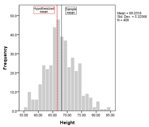
To add vertical reference lines at the mean (or another location), double-click on the plot to open the Chart Editor, then click Options > X Axis Reference Line . In the Properties window, you can enter a specific location on the x-axis for the vertical line, or you can choose to have the reference line at the mean or median of the sample data (using the sample data). Click Apply to make sure your new line is added to the chart. Here, we have added two reference lines: one at the sample mean (the solid black line), and the other at 66.5 (the dashed red line).

From the histogram, we can see that height is relatively symmetrically distributed about the mean, though there is a slightly longer right tail. The reference lines indicate that sample mean is slightly greater than the hypothesized mean, but not by a huge amount. It's possible that our test result could come back significant.

Running the Test

To run the One Sample t Test, click  Analyze > Compare Means > One-Sample T Test.  Move the variable Height to the Test Variable(s) area. In the Test Value field, enter 66.5.

If you are using SPSS Statistics 27 or later :

If you are using SPSS Statistics 26 or earlier :

Two sections (boxes) appear in the output: One-Sample Statistics and One-Sample Test . The first section, One-Sample Statistics , provides basic information about the selected variable, Height , including the valid (nonmissing) sample size ( n ), mean, standard deviation, and standard error. In this example, the mean height of the sample is 68.03 inches, which is based on 408 nonmissing observations.

The second section, One-Sample Test , displays the results most relevant to the One Sample t Test. 

A Test Value : The number we entered as the test value in the One-Sample T Test window.

B t Statistic : The test statistic of the one-sample t test, denoted t . In this example, t = 5.810. Note that t is calculated by dividing the mean difference (E) by the standard error mean (from the One-Sample Statistics box).

C df : The degrees of freedom for the test. For a one-sample t test, df = n - 1; so here, df = 408 - 1 = 407.

D Significance (One-Sided p and Two-Sided p): The p-values corresponding to one of the possible one-sided alternative hypotheses (in this case, µ Height > 66.5) and two-sided alternative hypothesis (µ Height ≠ 66.5), respectively. In our problem statement above, we were only interested in the two-sided alternative hypothesis.

E Mean Difference : The difference between the "observed" sample mean (from the One Sample Statistics box) and the "expected" mean (the specified test value (A)). The sign of the mean difference corresponds to the sign of the t value (B). The positive t value in this example indicates that the mean height of the sample is greater than the hypothesized value (66.5).

F Confidence Interval for the Difference : The confidence interval for the difference between the specified test value and the sample mean.

Decision and Conclusions

Recall that our hypothesized population value was 66.5 inches, the [approximate] average height of the overall adult population in the U.S. Since p < 0.001, we reject the null hypothesis that the mean height of students at this college is equal to the hypothesized population mean of 66.5 inches and conclude that the mean height is significantly different than 66.5 inches.

Based on the results, we can state the following:

• There is a significant difference in the mean height of the students at this college and the overall adult population in the U.S. ( p < .001).
• The average height of students at this college is about 1.5 inches taller than the U.S. adult population average (95% CI [1.013, 2.050]).
• << Previous: Pearson Correlation
• Next: Paired Samples t Test >>
• Last Updated: Jul 10, 2024 11:08 AM
• URL: https://libguides.library.kent.edu/SPSS

Street Address

Mailing address, quick links.

• How Are We Doing?
• Student Jobs

Information

• Accessibility
• Emergency Information
• For Our Alumni
• For the Media
• Jobs & Employment
• Life at KSU
• Privacy Statement
• Technology Support
• Website Feedback

• Skip to primary navigation
• Skip to main content
• Skip to primary sidebar

Statistical Methods and Data Analytics

What statistical analysis should I use? Statistical analyses using SPSS

Introduction.

This page shows how to perform a number of statistical tests using SPSS.  Each section gives a brief description of the aim of the statistical test, when it is used, an example showing the SPSS commands and SPSS (often abbreviated) output with a brief interpretation of the output. You can see the page Choosing the Correct Statistical Test for a table that shows an overview of when each test is appropriate to use.  In deciding which test is appropriate to use, it is important to consider the type of variables that you have (i.e., whether your variables are categorical, ordinal or interval and whether they are normally distributed), see What is the difference between categorical, ordinal and interval variables? for more information on this.

About the hsb data file

Most of the examples in this page will use a data file called hsb2, high school and beyond.  This data file contains 200 observations from a sample of high school students with demographic information about the students, such as their gender ( female ), socio-economic status ( ses ) and ethnic background ( race ). It also contains a number of scores on standardized tests, including tests of reading ( read ), writing ( write ), mathematics ( math ) and social studies ( socst ). You can get the hsb data file by clicking on hsb2 .

One sample t-test

A one sample t-test allows us to test whether a sample mean (of a normally distributed interval variable) significantly differs from a hypothesized value.  For example, using the hsb2 data file , say we wish to test whether the average writing score ( write ) differs significantly from 50.  We can do this as shown below. t-test  /testval = 50  /variable = write. The mean of the variable write for this particular sample of students is 52.775, which is statistically significantly different from the test value of 50.  We would conclude that this group of students has a significantly higher mean on the writing test than 50.

One sample median test

A one sample median test allows us to test whether a sample median differs significantly from a hypothesized value.  We will use the same variable, write , as we did in the one sample t-test example above, but we do not need to assume that it is interval and normally distributed (we only need to assume that write is an ordinal variable). nptests /onesample test (write) wilcoxon(testvalue = 50).

Binomial test

A one sample binomial test allows us to test whether the proportion of successes on a two-level categorical dependent variable significantly differs from a hypothesized value.  For example, using the hsb2 data file , say we wish to test whether the proportion of females ( female ) differs significantly from 50%, i.e., from .5.  We can do this as shown below. npar tests  /binomial (.5) = female. The results indicate that there is no statistically significant difference (p = .229).  In other words, the proportion of females in this sample does not significantly differ from the hypothesized value of 50%.

Chi-square goodness of fit

A chi-square goodness of fit test allows us to test whether the observed proportions for a categorical variable differ from hypothesized proportions.  For example, let’s suppose that we believe that the general population consists of 10% Hispanic, 10% Asian, 10% African American and 70% White folks.  We want to test whether the observed proportions from our sample differ significantly from these hypothesized proportions. npar test   /chisquare = race  /expected = 10 10 10 70. These results show that racial composition in our sample does not differ significantly from the hypothesized values that we supplied (chi-square with three degrees of freedom = 5.029, p = .170).

Two independent samples t-test

An independent samples t-test is used when you want to compare the means of a normally distributed interval dependent variable for two independent groups.  For example, using the hsb2 data file , say we wish to test whether the mean for write is the same for males and females. t-test groups = female(0 1)   /variables = write. Because the standard deviations for the two groups are similar (10.3 and 8.1), we will use the “equal variances assumed” test.  The results indicate that there is a statistically significant difference between the mean writing score for males and females (t = -3.734, p = .000).  In other words, females have a statistically significantly higher mean score on writing (54.99) than males (50.12). See also SPSS Learning Module: An overview of statistical tests in SPSS

Wilcoxon-Mann-Whitney test

The Wilcoxon-Mann-Whitney test is a non-parametric analog to the independent samples t-test and can be used when you do not assume that the dependent variable is a normally distributed interval variable (you only assume that the variable is at least ordinal).  You will notice that the SPSS syntax for the Wilcoxon-Mann-Whitney test is almost identical to that of the independent samples t-test.  We will use the same data file (the hsb2 data file ) and the same variables in this example as we did in the independent t-test example above and will not assume that write , our dependent variable, is normally distributed.

npar test /m-w = write by female(0 1). The results suggest that there is a statistically significant difference between the underlying distributions of the write scores of males and the write scores of females (z = -3.329, p = 0.001). See also FAQ: Why is the Mann-Whitney significant when the medians are equal?

Chi-square test

A chi-square test is used when you want to see if there is a relationship between two categorical variables.  In SPSS, the chisq option is used on the statistics subcommand of the crosstabs command to obtain the test statistic and its associated p-value.  Using the hsb2 data file , let’s see if there is a relationship between the type of school attended ( schtyp ) and students’ gender ( female ).  Remember that the chi-square test assumes that the expected value for each cell is five or higher. This assumption is easily met in the examples below.  However, if this assumption is not met in your data, please see the section on Fisher’s exact test below. crosstabs /tables = schtyp by female /statistic = chisq. These results indicate that there is no statistically significant relationship between the type of school attended and gender (chi-square with one degree of freedom = 0.047, p = 0.828). Let’s look at another example, this time looking at the linear relationship between gender ( female ) and socio-economic status ( ses ).  The point of this example is that one (or both) variables may have more than two levels, and that the variables do not have to have the same number of levels.  In this example, female has two levels (male and female) and ses has three levels (low, medium and high). crosstabs /tables = female by ses /statistic = chisq. Again we find that there is no statistically significant relationship between the variables (chi-square with two degrees of freedom = 4.577, p = 0.101). See also SPSS Learning Module: An Overview of Statistical Tests in SPSS

Fisher’s exact test

The Fisher’s exact test is used when you want to conduct a chi-square test but one or more of your cells has an expected frequency of five or less.  Remember that the chi-square test assumes that each cell has an expected frequency of five or more, but the Fisher’s exact test has no such assumption and can be used regardless of how small the expected frequency is. In SPSS unless you have the SPSS Exact Test Module, you can only perform a Fisher’s exact test on a 2×2 table, and these results are presented by default.  Please see the results from the chi squared example above.

One-way ANOVA

A one-way analysis of variance (ANOVA) is used when you have a categorical independent variable (with two or more categories) and a normally distributed interval dependent variable and you wish to test for differences in the means of the dependent variable broken down by the levels of the independent variable.  For example, using the hsb2 data file , say we wish to test whether the mean of write differs between the three program types ( prog ).  The command for this test would be: oneway write by prog. The mean of the dependent variable differs significantly among the levels of program type.  However, we do not know if the difference is between only two of the levels or all three of the levels.  (The F test for the Model is the same as the F test for prog because prog was the only variable entered into the model.  If other variables had also been entered, the F test for the Model would have been different from prog .)  To see the mean of write for each level of program type, means tables = write by prog. From this we can see that the students in the academic program have the highest mean writing score, while students in the vocational program have the lowest. See also SPSS Textbook Examples: Design and Analysis, Chapter 7 SPSS Textbook Examples: Applied Regression Analysis, Chapter 8 SPSS FAQ: How can I do ANOVA contrasts in SPSS? SPSS Library: Understanding and Interpreting Parameter Estimates in Regression and ANOVA

Kruskal Wallis test

The Kruskal Wallis test is used when you have one independent variable with two or more levels and an ordinal dependent variable. In other words, it is the non-parametric version of ANOVA and a generalized form of the Mann-Whitney test method since it permits two or more groups.  We will use the same data file as the one way ANOVA example above (the hsb2 data file ) and the same variables as in the example above, but we will not assume that write is a normally distributed interval variable. npar tests /k-w = write by prog (1,3). If some of the scores receive tied ranks, then a correction factor is used, yielding a slightly different value of chi-squared.  With or without ties, the results indicate that there is a statistically significant difference among the three type of programs.

Paired t-test

A paired (samples) t-test is used when you have two related observations (i.e., two observations per subject) and you want to see if the means on these two normally distributed interval variables differ from one another.  For example, using the hsb2 data file we will test whether the mean of read is equal to the mean of write . t-test pairs = read with write (paired). These results indicate that the mean of read is not statistically significantly different from the mean of write (t = -0.867, p = 0.387).

Wilcoxon signed rank sum test

The Wilcoxon signed rank sum test is the non-parametric version of a paired samples t-test.  You use the Wilcoxon signed rank sum test when you do not wish to assume that the difference between the two variables is interval and normally distributed (but you do assume the difference is ordinal). We will use the same example as above, but we will not assume that the difference between read and write is interval and normally distributed. npar test /wilcoxon = write with read (paired). The results suggest that there is not a statistically significant difference between read and write . If you believe the differences between read and write were not ordinal but could merely be classified as positive and negative, then you may want to consider a sign test in lieu of sign rank test.  Again, we will use the same variables in this example and assume that this difference is not ordinal. npar test /sign = read with write (paired). We conclude that no statistically significant difference was found (p=.556).

McNemar test

You would perform McNemar’s test if you were interested in the marginal frequencies of two binary outcomes. These binary outcomes may be the same outcome variable on matched pairs (like a case-control study) or two outcome variables from a single group.  Continuing with the hsb2 dataset used in several above examples, let us create two binary outcomes in our dataset: himath and hiread . These outcomes can be considered in a two-way contingency table.  The null hypothesis is that the proportion of students in the himath group is the same as the proportion of students in hiread group (i.e., that the contingency table is symmetric). compute himath = (math>60). compute hiread = (read>60). execute. crosstabs /tables=himath BY hiread /statistic=mcnemar /cells=count. McNemar’s chi-square statistic suggests that there is not a statistically significant difference in the proportion of students in the himath group and the proportion of students in the hiread group.

One-way repeated measures ANOVA

You would perform a one-way repeated measures analysis of variance if you had one categorical independent variable and a normally distributed interval dependent variable that was repeated at least twice for each subject.  This is the equivalent of the paired samples t-test, but allows for two or more levels of the categorical variable. This tests whether the mean of the dependent variable differs by the categorical variable.  We have an example data set called rb4wide , which is used in Kirk’s book Experimental Design.  In this data set, y is the dependent variable, a is the repeated measure and s is the variable that indicates the subject number. glm y1 y2 y3 y4 /wsfactor a(4). You will notice that this output gives four different p-values.  The output labeled “sphericity assumed”  is the p-value (0.000) that you would get if you assumed compound symmetry in the variance-covariance matrix.  Because that assumption is often not valid, the three other p-values offer various corrections (the Huynh-Feldt, H-F, Greenhouse-Geisser, G-G and Lower-bound).  No matter which p-value you use, our results indicate that we have a statistically significant effect of a at the .05 level. See also SPSS Textbook Examples from Design and Analysis: Chapter 16 SPSS Library: Advanced Issues in Using and Understanding SPSS MANOVA SPSS Code Fragment: Repeated Measures ANOVA

Repeated measures logistic regression

If you have a binary outcome measured repeatedly for each subject and you wish to run a logistic regression that accounts for the effect of multiple measures from single subjects, you can perform a repeated measures logistic regression.  In SPSS, this can be done using the GENLIN command and indicating binomial as the probability distribution and logit as the link function to be used in the model. The exercise data file contains 3 pulse measurements from each of 30 people assigned to 2 different diet regiments and 3 different exercise regiments. If we define a “high” pulse as being over 100, we can then predict the probability of a high pulse using diet regiment. GET FILE='C:mydatahttps://stats.idre.ucla.edu/wp-content/uploads/2016/02/exercise.sav'. GENLIN highpulse (REFERENCE=LAST) BY diet (order = DESCENDING) /MODEL diet DISTRIBUTION=BINOMIAL LINK=LOGIT /REPEATED SUBJECT=id CORRTYPE = EXCHANGEABLE. These results indicate that diet is not statistically significant (Wald Chi-Square = 1.562, p = 0.211).

Factorial ANOVA

A factorial ANOVA has two or more categorical independent variables (either with or without the interactions) and a single normally distributed interval dependent variable.  For example, using the hsb2 data file we will look at writing scores ( write ) as the dependent variable and gender ( female ) and socio-economic status ( ses ) as independent variables, and we will include an interaction of female by ses .  Note that in SPSS, you do not need to have the interaction term(s) in your data set.  Rather, you can have SPSS create it/them temporarily by placing an asterisk between the variables that will make up the interaction term(s). glm write by female ses. These results indicate that the overall model is statistically significant (F = 5.666, p = 0.00).  The variables female and ses are also statistically significant (F = 16.595, p = 0.000 and F = 6.611, p = 0.002, respectively).  However, that interaction between female and ses is not statistically significant (F = 0.133, p = 0.875). See also SPSS Textbook Examples from Design and Analysis: Chapter 10 SPSS FAQ: How can I do tests of simple main effects in SPSS? SPSS FAQ: How do I plot ANOVA cell means in SPSS? SPSS Library: An Overview of SPSS GLM

Friedman test

You perform a Friedman test when you have one within-subjects independent variable with two or more levels and a dependent variable that is not interval and normally distributed (but at least ordinal).  We will use this test to determine if there is a difference in the reading, writing and math scores.  The null hypothesis in this test is that the distribution of the ranks of each type of score (i.e., reading, writing and math) are the same.  To conduct a Friedman test, the data need to be in a long format.  SPSS handles this for you, but in other statistical packages you will have to reshape the data before you can conduct this test. npar tests /friedman = read write math. Friedman’s chi-square has a value of 0.645 and a p-value of 0.724 and is not statistically significant.  Hence, there is no evidence that the distributions of the three types of scores are different.

Ordered logistic regression

Ordered logistic regression is used when the dependent variable is ordered, but not continuous.  For example, using the hsb2 data file we will create an ordered variable called write3 .  This variable will have the values 1, 2 and 3, indicating a low, medium or high writing score.  We do not generally recommend categorizing a continuous variable in this way; we are simply creating a variable to use for this example.  We will use gender ( female ), reading score ( read ) and social studies score ( socst ) as predictor variables in this model.  We will use a logit link and on the print subcommand we have requested the parameter estimates, the (model) summary statistics and the test of the parallel lines assumption. if write ge 30 and write le 48 write3 = 1. if write ge 49 and write le 57 write3 = 2. if write ge 58 and write le 70 write3 = 3. execute. plum write3 with female read socst /link = logit /print = parameter summary tparallel. The results indicate that the overall model is statistically significant (p < .000), as are each of the predictor variables (p < .000).  There are two thresholds for this model because there are three levels of the outcome variable.  We also see that the test of the proportional odds assumption is non-significant (p = .563).  One of the assumptions underlying ordinal logistic (and ordinal probit) regression is that the relationship between each pair of outcome groups is the same.  In other words, ordinal logistic regression assumes that the coefficients that describe the relationship between, say, the lowest versus all higher categories of the response variable are the same as those that describe the relationship between the next lowest category and all higher categories, etc.  This is called the proportional odds assumption or the parallel regression assumption.  Because the relationship between all pairs of groups is the same, there is only one set of coefficients (only one model).  If this was not the case, we would need different models (such as a generalized ordered logit model) to describe the relationship between each pair of outcome groups. See also SPSS Data Analysis Examples: Ordered logistic regression SPSS Annotated Output:  Ordinal Logistic Regression

Factorial logistic regression

A factorial logistic regression is used when you have two or more categorical independent variables but a dichotomous dependent variable.  For example, using the hsb2 data file we will use female as our dependent variable, because it is the only dichotomous variable in our data set; certainly not because it common practice to use gender as an outcome variable.  We will use type of program ( prog ) and school type ( schtyp ) as our predictor variables.  Because prog is a categorical variable (it has three levels), we need to create dummy codes for it. SPSS will do this for you by making dummy codes for all variables listed after the keyword with .  SPSS will also create the interaction term; simply list the two variables that will make up the interaction separated by the keyword by . logistic regression female with prog schtyp prog by schtyp /contrast(prog) = indicator(1). The results indicate that the overall model is not statistically significant (LR chi2 = 3.147, p = 0.677).  Furthermore, none of the coefficients are statistically significant either.  This shows that the overall effect of prog is not significant. See also Annotated output for logistic regression

Correlation

A correlation is useful when you want to see the relationship between two (or more) normally distributed interval variables.  For example, using the hsb2 data file we can run a correlation between two continuous variables, read and write . correlations /variables = read write. In the second example, we will run a correlation between a dichotomous variable, female , and a continuous variable, write . Although it is assumed that the variables are interval and normally distributed, we can include dummy variables when performing correlations. correlations /variables = female write. In the first example above, we see that the correlation between read and write is 0.597.  By squaring the correlation and then multiplying by 100, you can determine what percentage of the variability is shared.  Let’s round 0.597 to be 0.6, which when squared would be .36, multiplied by 100 would be 36%.  Hence read shares about 36% of its variability with write .  In the output for the second example, we can see the correlation between write and female is 0.256.  Squaring this number yields .065536, meaning that female shares approximately 6.5% of its variability with write . See also Annotated output for correlation SPSS Learning Module: An Overview of Statistical Tests in SPSS SPSS FAQ: How can I analyze my data by categories? Missing Data in SPSS

Simple linear regression

Simple linear regression allows us to look at the linear relationship between one normally distributed interval predictor and one normally distributed interval outcome variable.  For example, using the hsb2 data file , say we wish to look at the relationship between writing scores ( write ) and reading scores ( read ); in other words, predicting write from read . regression variables = write read /dependent = write /method = enter. We see that the relationship between write and read is positive (.552) and based on the t-value (10.47) and p-value (0.000), we would conclude this relationship is statistically significant.  Hence, we would say there is a statistically significant positive linear relationship between reading and writing. See also Regression With SPSS: Chapter 1 – Simple and Multiple Regression Annotated output for regression SPSS Textbook Examples: Introduction to the Practice of Statistics, Chapter 10 SPSS Textbook Examples: Regression with Graphics, Chapter 2 SPSS Textbook Examples: Applied Regression Analysis, Chapter 5

Non-parametric correlation

A Spearman correlation is used when one or both of the variables are not assumed to be normally distributed and interval (but are assumed to be ordinal). The values of the variables are converted in ranks and then correlated.  In our example, we will look for a relationship between read and write .  We will not assume that both of these variables are normal and interval. nonpar corr /variables = read write /print = spearman. The results suggest that the relationship between read and write (rho = 0.617, p = 0.000) is statistically significant.

Simple logistic regression

Logistic regression assumes that the outcome variable is binary (i.e., coded as 0 and 1).  We have only one variable in the hsb2 data file that is coded 0 and 1, and that is female .  We understand that female is a silly outcome variable (it would make more sense to use it as a predictor variable), but we can use female as the outcome variable to illustrate how the code for this command is structured and how to interpret the output.  The first variable listed after the logistic command is the outcome (or dependent) variable, and all of the rest of the variables are predictor (or independent) variables.  In our example, female will be the outcome variable, and read will be the predictor variable.  As with OLS regression, the predictor variables must be either dichotomous or continuous; they cannot be categorical. logistic regression female with read. The results indicate that reading score ( read ) is not a statistically significant predictor of gender (i.e., being female), Wald = .562, p = 0.453. Likewise, the test of the overall model is not statistically significant, LR chi-squared – 0.56, p = 0.453. See also Annotated output for logistic regression SPSS Library: What kind of contrasts are these?

Multiple regression

Multiple regression is very similar to simple regression, except that in multiple regression you have more than one predictor variable in the equation.  For example, using the hsb2 data file we will predict writing score from gender ( female ), reading, math, science and social studies ( socst ) scores. regression variable = write female read math science socst /dependent = write /method = enter. The results indicate that the overall model is statistically significant (F = 58.60, p = 0.000).  Furthermore, all of the predictor variables are statistically significant except for read . See also Regression with SPSS: Chapter 1 – Simple and Multiple Regression Annotated output for regression SPSS Frequently Asked Questions SPSS Textbook Examples: Regression with Graphics, Chapter 3 SPSS Textbook Examples: Applied Regression Analysis

Analysis of covariance

Analysis of covariance is like ANOVA, except in addition to the categorical predictors you also have continuous predictors as well.  For example, the one way ANOVA example used write as the dependent variable and prog as the independent variable.  Let’s add read as a continuous variable to this model, as shown below. glm write with read by prog. The results indicate that even after adjusting for reading score ( read ), writing scores still significantly differ by program type ( prog ), F = 5.867, p = 0.003. See also SPSS Textbook Examples from Design and Analysis: Chapter 14 SPSS Library: An Overview of SPSS GLM SPSS Library: How do I handle interactions of continuous and categorical variables?

Multiple logistic regression

Multiple logistic regression is like simple logistic regression, except that there are two or more predictors.  The predictors can be interval variables or dummy variables, but cannot be categorical variables.  If you have categorical predictors, they should be coded into one or more dummy variables. We have only one variable in our data set that is coded 0 and 1, and that is female .  We understand that female is a silly outcome variable (it would make more sense to use it as a predictor variable), but we can use female as the outcome variable to illustrate how the code for this command is structured and how to interpret the output.  The first variable listed after the logistic regression command is the outcome (or dependent) variable, and all of the rest of the variables are predictor (or independent) variables (listed after the keyword with ).  In our example, female will be the outcome variable, and read and write will be the predictor variables. logistic regression female with read write. These results show that both read and write are significant predictors of female . See also Annotated output for logistic regression SPSS Textbook Examples: Applied Logistic Regression, Chapter 2 SPSS Code Fragments: Graphing Results in Logistic Regression

Discriminant analysis

Discriminant analysis is used when you have one or more normally distributed interval independent variables and a categorical dependent variable.  It is a multivariate technique that considers the latent dimensions in the independent variables for predicting group membership in the categorical dependent variable.  For example, using the hsb2 data file , say we wish to use read , write and math scores to predict the type of program a student belongs to ( prog ). discriminate groups = prog(1, 3) /variables = read write math. Clearly, the SPSS output for this procedure is quite lengthy, and it is beyond the scope of this page to explain all of it.  However, the main point is that two canonical variables are identified by the analysis, the first of which seems to be more related to program type than the second. See also discriminant function analysis SPSS Library: A History of SPSS Statistical Features

One-way MANOVA

MANOVA (multivariate analysis of variance) is like ANOVA, except that there are two or more dependent variables. In a one-way MANOVA, there is one categorical independent variable and two or more dependent variables. For example, using the hsb2 data file , say we wish to examine the differences in read , write and math broken down by program type ( prog ). glm read write math by prog. The students in the different programs differ in their joint distribution of read , write and math . See also SPSS Library: Advanced Issues in Using and Understanding SPSS MANOVA GLM: MANOVA and MANCOVA SPSS Library: MANOVA and GLM

Multivariate multiple regression

Multivariate multiple regression is used when you have two or more dependent variables that are to be predicted from two or more independent variables.  In our example using the hsb2 data file , we will predict write and read from female , math , science and social studies ( socst ) scores. glm write read with female math science socst. These results show that all of  the variables in the model have a statistically significant relationship with the joint distribution of write and read .

Canonical correlation

Canonical correlation is a multivariate technique used to examine the relationship between two groups of variables.  For each set of variables, it creates latent variables and looks at the relationships among the latent variables. It assumes that all variables in the model are interval and normally distributed.  SPSS requires that each of the two groups of variables be separated by the keyword with .  There need not be an equal number of variables in the two groups (before and after the with ). manova read write with math science /discrim. * * * * * * A n a l y s i s o f V a r i a n c e -- design 1 * * * * * * EFFECT .. WITHIN CELLS Regression Multivariate Tests of Significance (S = 2, M = -1/2, N = 97 ) Test Name Value Approx. F Hypoth. DF Error DF Sig. of F Pillais .59783 41.99694 4.00 394.00 .000 Hotellings 1.48369 72.32964 4.00 390.00 .000 Wilks .40249 56.47060 4.00 392.00 .000 Roys .59728 Note.. F statistic for WILKS' Lambda is exact. - - - - - - - - - - - - - - - - - - - - - - - - - - - - - - - - - - - - - EFFECT .. WITHIN CELLS Regression (Cont.) Univariate F-tests with (2,197) D. F. Variable Sq. Mul. R Adj. R-sq. Hypoth. MS Error MS F READ .51356 .50862 5371.66966 51.65523 103.99081 WRITE .43565 .42992 3894.42594 51.21839 76.03569 Variable Sig. of F READ .000 WRITE .000 - - - - - - - - - - - - - - - - - - - - - - - - - - - - - - - - - - - - - Raw canonical coefficients for DEPENDENT variables Function No. Variable 1 READ .063 WRITE .049 - - - - - - - - - - - - - - - - - - - - - - - - - - - - - - - - - - - - - Standardized canonical coefficients for DEPENDENT variables Function No. Variable 1 READ .649 WRITE .467 * * * * * * A n a l y s i s o f V a r i a n c e -- design 1 * * * * * * Correlations between DEPENDENT and canonical variables Function No. Variable 1 READ .927 WRITE .854 - - - - - - - - - - - - - - - - - - - - - - - - - - - - - - - - - - - - - Variance in dependent variables explained by canonical variables CAN. VAR. Pct Var DE Cum Pct DE Pct Var CO Cum Pct CO 1 79.441 79.441 47.449 47.449 - - - - - - - - - - - - - - - - - - - - - - - - - - - - - - - - - - - - - Raw canonical coefficients for COVARIATES Function No. COVARIATE 1 MATH .067 SCIENCE .048 - - - - - - - - - - - - - - - - - - - - - - - - - - - - - - - - - - - - - Standardized canonical coefficients for COVARIATES CAN. VAR. COVARIATE 1 MATH .628 SCIENCE .478 - - - - - - - - - - - - - - - - - - - - - - - - - - - - - - - - - - - - - Correlations between COVARIATES and canonical variables CAN. VAR. Covariate 1 MATH .929 SCIENCE .873 * * * * * * A n a l y s i s o f V a r i a n c e -- design 1 * * * * * * Variance in covariates explained by canonical variables CAN. VAR. Pct Var DE Cum Pct DE Pct Var CO Cum Pct CO 1 48.544 48.544 81.275 81.275 - - - - - - - - - - - - - - - - - - - - - - - - - - - - - - - - - - - - - Regression analysis for WITHIN CELLS error term --- Individual Univariate .9500 confidence intervals Dependent variable .. READ reading score COVARIATE B Beta Std. Err. t-Value Sig. of t MATH .48129 .43977 .070 6.868 .000 SCIENCE .36532 .35278 .066 5.509 .000 COVARIATE Lower -95% CL- Upper MATH .343 .619 SCIENCE .235 .496 Dependent variable .. WRITE writing score COVARIATE B Beta Std. Err. t-Value Sig. of t MATH .43290 .42787 .070 6.203 .000 SCIENCE .28775 .30057 .066 4.358 .000 COVARIATE Lower -95% CL- Upper MATH .295 .571 SCIENCE .158 .418 - - - - - - - - - - - - - - - - - - - - - - - - - - - - - - - - - - - - - * * * * * * A n a l y s i s o f V a r i a n c e -- design 1 * * * * * * EFFECT .. CONSTANT Multivariate Tests of Significance (S = 1, M = 0, N = 97 ) Test Name Value Exact F Hypoth. DF Error DF Sig. of F Pillais .11544 12.78959 2.00 196.00 .000 Hotellings .13051 12.78959 2.00 196.00 .000 Wilks .88456 12.78959 2.00 196.00 .000 Roys .11544 Note.. F statistics are exact. - - - - - - - - - - - - - - - - - - - - - - - - - - - - - - - - - - - - - EFFECT .. CONSTANT (Cont.) Univariate F-tests with (1,197) D. F. Variable Hypoth. SS Error SS Hypoth. MS Error MS F Sig. of F READ 336.96220 10176.0807 336.96220 51.65523 6.52329 .011 WRITE 1209.88188 10090.0231 1209.88188 51.21839 23.62202 .000 - - - - - - - - - - - - - - - - - - - - - - - - - - - - - - - - - - - - - EFFECT .. CONSTANT (Cont.) Raw discriminant function coefficients Function No. Variable 1 READ .041 WRITE .124 - - - - - - - - - - - - - - - - - - - - - - - - - - - - - - - - - - - - - Standardized discriminant function coefficients Function No. Variable 1 READ .293 WRITE .889 - - - - - - - - - - - - - - - - - - - - - - - - - - - - - - - - - - - - - Estimates of effects for canonical variables Canonical Variable Parameter 1 1 2.196 * * * * * * A n a l y s i s o f V a r i a n c e -- design 1 * * * * * * EFFECT .. CONSTANT (Cont.) Correlations between DEPENDENT and canonical variables Canonical Variable Variable 1 READ .504 WRITE .959 - - - - - - - - - - - - - - - - - - - - - - - - - - - - - - - - - - - - - The output above shows the linear combinations corresponding to the first canonical correlation.  At the bottom of the output are the two canonical correlations. These results indicate that the first canonical correlation is .7728.  The F-test in this output tests the hypothesis that the first canonical correlation is equal to zero.  Clearly, F = 56.4706 is statistically significant.  However, the second canonical correlation of .0235 is not statistically significantly different from zero (F = 0.1087, p = 0.7420).

Factor analysis

Factor analysis is a form of exploratory multivariate analysis that is used to either reduce the number of variables in a model or to detect relationships among variables.  All variables involved in the factor analysis need to be interval and are assumed to be normally distributed.  The goal of the analysis is to try to identify factors which underlie the variables.  There may be fewer factors than variables, but there may not be more factors than variables.  For our example using the hsb2 data file , let’s suppose that we think that there are some common factors underlying the various test scores.  We will include subcommands for varimax rotation and a plot of the eigenvalues.  We will use a principal components extraction and will retain two factors. (Using these options will make our results compatible with those from SAS and Stata and are not necessarily the options that you will want to use.) factor /variables read write math science socst /criteria factors(2) /extraction pc /rotation varimax /plot eigen. Communality (which is the opposite of uniqueness) is the proportion of variance of the variable (i.e., read ) that is accounted for by all of the factors taken together, and a very low communality can indicate that a variable may not belong with any of the factors.  The scree plot may be useful in determining how many factors to retain.  From the component matrix table, we can see that all five of the test scores load onto the first factor, while all five tend to load not so heavily on the second factor.  The purpose of rotating the factors is to get the variables to load either very high or very low on each factor.  In this example, because all of the variables loaded onto factor 1 and not on factor 2, the rotation did not aid in the interpretation. Instead, it made the results even more difficult to interpret. See also SPSS FAQ: What does Cronbach’s alpha mean?

Your Name (required)

Your Email (must be a valid email for us to receive the report!)

Comment/Error Report (required)

How to cite this page

• © 2024 UC REGENTS

Have a language expert improve your writing

Run a free plagiarism check in 10 minutes, generate accurate citations for free.

• Knowledge Base
• Choosing the Right Statistical Test | Types & Examples

Choosing the Right Statistical Test | Types & Examples

Published on January 28, 2020 by Rebecca Bevans . Revised on June 22, 2023.

Statistical tests are used in hypothesis testing . They can be used to:

• determine whether a predictor variable has a statistically significant relationship with an outcome variable.
• estimate the difference between two or more groups.

Statistical tests assume a null hypothesis of no relationship or no difference between groups. Then they determine whether the observed data fall outside of the range of values predicted by the null hypothesis.

If you already know what types of variables you’re dealing with, you can use the flowchart to choose the right statistical test for your data.

Statistical tests flowchart

Table of contents

What does a statistical test do, when to perform a statistical test, choosing a parametric test: regression, comparison, or correlation, choosing a nonparametric test, flowchart: choosing a statistical test, other interesting articles, frequently asked questions about statistical tests.

Statistical tests work by calculating a test statistic – a number that describes how much the relationship between variables in your test differs from the null hypothesis of no relationship.

It then calculates a p value (probability value). The p -value estimates how likely it is that you would see the difference described by the test statistic if the null hypothesis of no relationship were true.

If the value of the test statistic is more extreme than the statistic calculated from the null hypothesis, then you can infer a statistically significant relationship between the predictor and outcome variables.

If the value of the test statistic is less extreme than the one calculated from the null hypothesis, then you can infer no statistically significant relationship between the predictor and outcome variables.

Here's why students love Scribbr's proofreading services

Discover proofreading & editing

You can perform statistical tests on data that have been collected in a statistically valid manner – either through an experiment , or through observations made using probability sampling methods .

For a statistical test to be valid , your sample size needs to be large enough to approximate the true distribution of the population being studied.

To determine which statistical test to use, you need to know:

• whether your data meets certain assumptions.
• the types of variables that you’re dealing with.

Statistical assumptions

Statistical tests make some common assumptions about the data they are testing:

• Independence of observations (a.k.a. no autocorrelation): The observations/variables you include in your test are not related (for example, multiple measurements of a single test subject are not independent, while measurements of multiple different test subjects are independent).
• Homogeneity of variance : the variance within each group being compared is similar among all groups. If one group has much more variation than others, it will limit the test’s effectiveness.
• Normality of data : the data follows a normal distribution (a.k.a. a bell curve). This assumption applies only to quantitative data .

If your data do not meet the assumptions of normality or homogeneity of variance, you may be able to perform a nonparametric statistical test , which allows you to make comparisons without any assumptions about the data distribution.

If your data do not meet the assumption of independence of observations, you may be able to use a test that accounts for structure in your data (repeated-measures tests or tests that include blocking variables).

Types of variables

The types of variables you have usually determine what type of statistical test you can use.

Quantitative variables represent amounts of things (e.g. the number of trees in a forest). Types of quantitative variables include:

• Continuous (aka ratio variables): represent measures and can usually be divided into units smaller than one (e.g. 0.75 grams).
• Discrete (aka integer variables): represent counts and usually can’t be divided into units smaller than one (e.g. 1 tree).

Categorical variables represent groupings of things (e.g. the different tree species in a forest). Types of categorical variables include:

• Ordinal : represent data with an order (e.g. rankings).
• Nominal : represent group names (e.g. brands or species names).
• Binary : represent data with a yes/no or 1/0 outcome (e.g. win or lose).

Choose the test that fits the types of predictor and outcome variables you have collected (if you are doing an experiment , these are the independent and dependent variables ). Consult the tables below to see which test best matches your variables.

Parametric tests usually have stricter requirements than nonparametric tests, and are able to make stronger inferences from the data. They can only be conducted with data that adheres to the common assumptions of statistical tests.

The most common types of parametric test include regression tests, comparison tests, and correlation tests.

Regression tests

Regression tests look for cause-and-effect relationships . They can be used to estimate the effect of one or more continuous variables on another variable.

Comparison tests

Comparison tests look for differences among group means . They can be used to test the effect of a categorical variable on the mean value of some other characteristic.

T-tests are used when comparing the means of precisely two groups (e.g., the average heights of men and women). ANOVA and MANOVA tests are used when comparing the means of more than two groups (e.g., the average heights of children, teenagers, and adults).

Correlation tests

Correlation tests check whether variables are related without hypothesizing a cause-and-effect relationship.

These can be used to test whether two variables you want to use in (for example) a multiple regression test are autocorrelated.

Non-parametric tests don’t make as many assumptions about the data, and are useful when one or more of the common statistical assumptions are violated. However, the inferences they make aren’t as strong as with parametric tests.

Prevent plagiarism. Run a free check.

This flowchart helps you choose among parametric tests. For nonparametric alternatives, check the table above.

If you want to know more about statistics , methodology , or research bias , make sure to check out some of our other articles with explanations and examples.

• Normal distribution
• Descriptive statistics
• Measures of central tendency
• Correlation coefficient
• Null hypothesis

Methodology

• Cluster sampling
• Stratified sampling
• Types of interviews
• Cohort study
• Thematic analysis

Research bias

• Implicit bias
• Cognitive bias
• Survivorship bias
• Availability heuristic
• Nonresponse bias
• Regression to the mean

Statistical tests commonly assume that:

• the data are normally distributed
• the groups that are being compared have similar variance
• the data are independent

If your data does not meet these assumptions you might still be able to use a nonparametric statistical test , which have fewer requirements but also make weaker inferences.

A test statistic is a number calculated by a  statistical test . It describes how far your observed data is from the  null hypothesis  of no relationship between  variables or no difference among sample groups.

The test statistic tells you how different two or more groups are from the overall population mean , or how different a linear slope is from the slope predicted by a null hypothesis . Different test statistics are used in different statistical tests.

Statistical significance is a term used by researchers to state that it is unlikely their observations could have occurred under the null hypothesis of a statistical test . Significance is usually denoted by a p -value , or probability value.

Statistical significance is arbitrary – it depends on the threshold, or alpha value, chosen by the researcher. The most common threshold is p < 0.05, which means that the data is likely to occur less than 5% of the time under the null hypothesis .

When the p -value falls below the chosen alpha value, then we say the result of the test is statistically significant.

Quantitative variables are any variables where the data represent amounts (e.g. height, weight, or age).

Categorical variables are any variables where the data represent groups. This includes rankings (e.g. finishing places in a race), classifications (e.g. brands of cereal), and binary outcomes (e.g. coin flips).

You need to know what type of variables you are working with to choose the right statistical test for your data and interpret your results .

Discrete and continuous variables are two types of quantitative variables :

• Discrete variables represent counts (e.g. the number of objects in a collection).
• Continuous variables represent measurable amounts (e.g. water volume or weight).

Cite this Scribbr article

If you want to cite this source, you can copy and paste the citation or click the “Cite this Scribbr article” button to automatically add the citation to our free Citation Generator.

Bevans, R. (2023, June 22). Choosing the Right Statistical Test | Types & Examples. Scribbr. Retrieved August 10, 2024, from https://www.scribbr.com/statistics/statistical-tests/

Is this article helpful?

Rebecca Bevans

Other students also liked, hypothesis testing | a step-by-step guide with easy examples, test statistics | definition, interpretation, and examples, normal distribution | examples, formulas, & uses, what is your plagiarism score.

Hypothesis test in SPSS

April 16, 2019

For the purpose of this tutorial, I’m gonna be using the sample data set demo.sav , available under installdir/IBM/SPSS/Statistics/[version]/Samples/[lang] , in my case, on Windows that would be C:\Program Files\IBM\SPSS\Statistics\25\Samples\English .

• If you haven’t already make sure to open the sample data set demo.sav (this data set is incidentally available in many different formats, such as txt and xlsx ).
• Click on Analyze>>Nonparametric Tests>>One Sample…
• In the resulting window, choose Automatically compare observed data to hypothesized .
• Click on the tab Fields .
• Depending on the version of SPSS, either all variables or just the categorical ones are available in the right column, Test Fields . However, for the purpose of this tutorial we’ll perform a one-sample binomial test so keep Gender which is a nominal variable and remove the rest (if the column Test Fields isn’t populated just add Gender and you’re good to go). The following hypothesis test will consequently answer the question What proportion of this sample is male or female?
• Under the next tab, Settings , there is the possibility to customize Significance level and Confidence interval. However the defaults are already at 0.05 and 95% respectively which will do just fine.
• Click Run .
• The result is a single nonparametric test. In the resulting table the null hypothesis is stated as The categories defined by Gender = Female and Male occur with probabilities 0.5 and 0.5 . The significance for this test SPSS calculated as 0.608 which is quite high and consequently the recommendation is to retain the null hypothesis (as the significance level is 0.05), which in this case means that the proportions male and female are about equal.

Which Statistical Test Should I Use?

• Univariate Tests
• Within-Subjects Tests
• Between-Subjects Tests
• Association Measures
• Prediction Analyses
• Classification Analyses

Finding the appropriate statistical test is easy if you're aware of

• the basic type of test you're looking for and
• the measurement levels of the variables involved.

For each type and measurement level, this tutorial immediately points out the right statistical test. We'll also briefly define the 6 basic types of tests and illustrate them with simple examples.

1. Overview Univariate Tests

Univariate Tests - Quick Definition

Univariate tests are tests that involve only 1 variable. Univariate tests either test if

• some population parameter -usually a mean or median - is equal to some hypothesized value or
• some population distribution is equal to some function, often the normal distribution .

A textbook example is a one sample t-test : it tests if a population mean -a parameter- is equal to some value x . This test involves only 1 variable (even if there's many more in your data file).

2. Overview Within-Subjects Tests

Within-Subjects Tests - Quick Definition

Within-subjects tests compare 2+ variables measured on the same subjects (often people). An example is repeated measures ANOVA : it tests if 3+ variables measured on the same subjects have equal population means.

Within-subjects tests are also known as

• paired samples tests (as in a paired samples t-test ) or
• related samples tests.

3. Overview Between-Subjects Tests

Between-Subjects Tests - Quick Definition

Between-subjects tests examine if 2+ subpopulations are identical with regard to

• a parameter (population mean, standard deviation or proportion) or
• a distribution .

The best known example is a one-way ANOVA as illustrated below. Note that the subpopulations are represented by subsamples -groups of observations indicated by some categorical variable.

“Between-subjects” tests are also known as “ independent samples ” tests, such as the independent samples t-test . “Independent samples” means that subsamples don't overlap: each observation belongs to only 1 subsample.

4. Overview Association Measures

Association Measures - Quick Definition

Association measures are numbers that indicate to what extent 2 variables are associated. The best known association measure is the Pearson correlation : a number that tells us to what extent 2 quantitative variables are linearly related. The illustration below visualizes correlations as scatterplots.

5. Overview Prediction Analyses

Prediction Analyses - Quick Definition

Prediction tests examine how and to what extent a variable can be predicted from 1+ other variables. The simplest example is simple linear regression as illustrated below.

Prediction analyses sometimes quietly assume causality : whatever predicts some variable is often thought to affect this variable. Depending on the contents of an analysis, causality may or may not be plausible. Keep in mind, however, that the analyses listed below don't prove causality.

6. Classification Analyses

Classification analyses attempt to identify and describe groups of observations or variables. The 2 main types of classification analysis are

• factor analysis for finding groups of variables (“factors”) and
• cluster analysis for finding groups of observations (“clusters”).

Factor analysis is based on correlations or covariances . Groups of variables that correlate strongly are assumed to measure similar underlying factors -sometimes called “constructs”. The basic idea is illustrated below.

Cluster analysis is based on distances among observations -often people. Groups of observations with small distances among them are assumed to represent clusters such as market segments.

Right. So that'll do for a basic overview. Hope you found this guide helpful! And last but not least,

thanks for reading!

Tell us what you think!

This tutorial has 18 comments:.

By Aidarous on October 12th, 2022

By ozman on July 29th, 2023

I enjoy reading your tutorials and always look forward to the latest instalment.

I have one small (trivial) comment on the tutorial titled "which statistical test...".

In the last 2 tables (Factor, Cluster) you have "Madelyn" listed twice as a first name. I realize that there may be two Madelyns with different last names, but in the absence of information on last name, one concludes that this is the same person (a repeated measure), which may cause some confusion for the reader. Perhaps a different first name is warranted.

Thanks and keep up the good work.

By Ruben Geert van den Berg on July 29th, 2023

Thanks for your suggestion, I'll implement it in the next update.

These are simulated data but "Madelyn" appearing twice is indeed somewhat unfortunate.

Great catch, really. If all analysts had this level of "eye for detail", there wouldn't be much of a replication crisis in the social sciences.

Kind regards from Amsterdam!

Ruben SPSS tutorials

Hypothesis Testing: SPSS (2.1)

Introduction: Hypothesis Testing: SPSS (2.1)

Recommendations

Woodworking Contest

Farm to Table Contest

Art and Sculpture Contest

Stack Exchange Network

Stack Exchange network consists of 183 Q&A communities including Stack Overflow , the largest, most trusted online community for developers to learn, share their knowledge, and build their careers.

Q&A for work

Connect and share knowledge within a single location that is structured and easy to search.

Which statistical test to use for Likert scale questionaire

I need help on determining what tests to use in SPSS. Let me provide some background on my research:

• I am doing a research on system automation of leave management in a company (which is still using a manual paper form to apply for leave).
• My hypothesis validates the automation of the different processes (independent variables) on the overall improvement of the leave management process (dependent). My control variables are age, gender and dept.
• I have developed a prototype of a system and provided a questionnaire in the form of a 5-point Likert scale to the participant. (Strongly Agree, Agree, Neutral, Disagree, Strongly Disagree).
• The questions measures their response on the statement provided on the test evaluation of the system. These questions are categorised based on the hypothesis.

Where do I start?

• hypothesis-testing

3 Answers 3

It sounds like your response (or "dependent") variable is perception of improvement eg individuals' response to a statement "leave management is better now than it was" (agree/disagree etc). Assuming this is the case, you first need to clarify that you don't really test the hypothesis of improvement of the system, only retrospective perceptions of it.

Putting that aside and given the data that you apparently have, it sounds like the technique you need is ordinal regression . A quick google suggests this is possible in SPSS (I'm not an SPSS user so I won't try to recommend any of the links).

• $\begingroup$ Yes, you are right - I would like to test the users response to the statements as the perception of the improvement. Is there any other tests that I can use? Which test to use to to know whether there is a relationship between the statements and the age, gender, dept the users belongs to? $\endgroup$ –  youngmoon Commented Mar 27, 2013 at 9:01

"Where do I start?"

You should always start a research study by clearly defining your objective (supported by literature review) and then identify your hypothesis to be tested, if any. Based on these, you should collect data to analyze. What's your objective?

• To study the factors affecting the perceptions of users about overall improvement of the leave management process by automation of the different processes.
• To study the impact of demographic characteristics on these factors

If these are your objectives, then you can use the following techniques:

Factor Analysis to identify the factors (for objective -1)

Three ANOVA tests corresponding to each demographic characteristic (age, gender, dept) [Note: for categories of input variable like gender (M/F), t- test can also be used, the results would be the same.

Try Fishers exact test to assess the association between the dependent and independent variables; whenever there is an association go for Contingency coefficient to see the strength of association between the variables. Go for correlation coefficient to see the relationship between demographic variables and perception improvement. But you have to do scoring for perception improvement

Your Answer

Sign up or log in, post as a guest.

Required, but never shown

By clicking “Post Your Answer”, you agree to our terms of service and acknowledge you have read our privacy policy .

Not the answer you're looking for? Browse other questions tagged hypothesis-testing spss likert or ask your own question .

• Featured on Meta
• Introducing an accessibility dashboard and some upcoming changes to display...
• We've made changes to our Terms of Service & Privacy Policy - July 2024
• Announcing a change to the data-dump process

Hot Network Questions

• When can a citizen's arrest of an Interpol fugitive be legal in Washington D.C.?
• Strategies for handling Maternity leave the last two weeks of the semester
• Can a Hall sensor be tested with just basic test gear?
• What was R' Chanina's Technique to Revive R' Yochanan?
• commands execution based on file size fails with no apparent issues
• Weird lines in the Aeneid (Book I, lines 444-445)
• Can an elf and a firbolg breed?
• Why is the completely dark disk of the Moon visible on a new moon if the lunar orbit is at an angle to the Earth’s?
• How to find a simplified sinogram in a paper dictionary
• How important is a "no reflection" strategy for 1 Hz systems?
• Why do most published papers hit the maximum page limit exactly?
• Short story probably in Omni magazine in the 1980s set in a cyberpunk bar… but it's 1899 or so
• Use of initialisms such as DMG, PHB and MM in third-party content
• Which Boolean Math mode should I use?
• SSH connectivity issues between local server and remote server
• How much does flight help the ranger?
• Why isn't the Liar's Paradox just accepted to be complete nonsense?
• Do the merits of an exegesis relying on texts unavailable to the author depend upon whether the unavailable texts were invented or not-yet-existent?
• Tips/strategies to managing my debt
• MPs assuming office on the day of the election
• What type of concept is "mad scientist"?
• sed (or awk): print captured group or placeholder if it doesn't exist
• Why do we sometimes use the concept of limits but sometimes don't forget similar kind of problems?
• In relation to the Tandy TRS-80 Model 1 and Model III, what are "ISAM" and "PDS"?

Pardon Our Interruption

As you were browsing something about your browser made us think you were a bot. There are a few reasons this might happen:

• You've disabled JavaScript in your web browser.
• You're a power user moving through this website with super-human speed.
• You've disabled cookies in your web browser.
• A third-party browser plugin, such as Ghostery or NoScript, is preventing JavaScript from running. Additional information is available in this support article .

To regain access, please make sure that cookies and JavaScript are enabled before reloading the page.